The Hash, the Merkle Tree, and Bitcoin

Although cryptocurrencies have been mainstream for quite a while, I still think the popular press has not done a great job explaining the details of how they work. There are several ideas behind a cryptocurrency like Bitcoin but the main one is the concept of a cryptographic hash. In simple terms, a hash is a way to transform an input sequence of characters (i.e. a string) into an output string such that it is hard to recreate the input string from the output string. A transformation with this property is called a one-way function. It is a machine where you get an output from an input but you can’t get the input from the output and there does not exist any other machine that can get the input from the output. A hash is a one-way function where the output has a standard form, e.g. 64 characters long. So if each character is a bit, e.g. 0 or 1, then there are different possible hashes. What makes hashes useful are two properties. The first, as mentioned, is that it is a one-way function and the second is that two different inputs do not give the same hash, called collision avoidance. There have been decades of work on figuring out how to do this and institutions like the US National Institutes of Standards and Technology (NIST) actually publish hash standards like SHA-2.

Hashes are an important part of your life. If a company is responsible, then only the hash of your password is stored on their servers, and when you type your password into a website, it goes through the hashing function and the hash is checked against the stored version. That way, if there is security breach, only the hash list is stolen. If the company is very responsible, then your name and all of your information is also only stored in hash form. Part of the problem with past security breaches is that the companies stored actual information instead of hashed information. However, if you use the same password on different websites then the hash would be same if the same standard was used. Some really careful companies will “salt” your password by adding a random string to it (that is hopefullly stored separately) before hashing. Or they will rehash your hash with salt. If you had a perfect hash, then the only way to break it would be to guess different inputs and see if it matches the desired output. The so-called complex math problem that Bitcoin solves before validating a transaction (and getting a reward) is finding a hash with a certain property but more on this later.

Now, one of the problems with hashing is that you need to deal with inputs of various sizes but you want the output to have a single uniform size. So even though a hash could have enough information capacity (i.e. entropy) to encode all of the world’s information ten times over, it is computationally inconvenient to just feed the complete text of Hamlet directly into a single one-way function. This is where the concept of a Merkle tree becomes important. You start with some one-way function that takes inputs of some fixed length and it scrambles the characters in some way that is not easily reversible. If the input string is too short then you just add extra characters (called padding) but if it is too long you need to do something else. The way a Merkle tree works is to break the text into chunks of uniform size. It then hashes the first chunk, adds that to the next chunk, hash the result and repeat until you have included all the chunks. This repeated recursive hashing is the secret sauce of crypto-currencies.

Bitcoin tried to create a completely decentralized digital currency that could be secure and trusted. For a regular currency like the US dollar, the thing you are most concerned about is that the dollar you receive is not counterfeit. The way that problem is solved is to make the manufacturing process of dollar bills very difficult to reproduce. So the dollar uses special paper with special marks and threads and special fonts and special ink. There are laws against making photocopiers with a higher resolution than the smallest print on a US bill to safeguard against counterfeiting. A problem with digital currencies is that you need to prevent double spending. The way this is historically solved is to have all transactions validated by a central authority.

Bitcoin solves these problems in a decentralized system by using a public ledger, called a blockchain that is time stamped, immutable and verifiable. The block chain keeps track of every Bitcoin transaction. So if you wanted to transfer one Bitcoin to someone else then the blockchain would show that your private Bitcoin ID has one less Bitcoin and the ID of the person you transferred to would have one extra Bitcoin. It is called a blockchain because each transaction (or set of transactions) is recorded into a block, the blocks are sequential, and each block contains a hash of the previous block. To validate a transaction you would need to validate each transaction leading up to the last block to validate that the hash on each block is correct. Thus the blockchain is a Merkle tree ledger where each entry is time stamped, immutable, and verifiable. If you want to change a block you need to change all the blocks before it.

However, the blockchain is not decentralized on its own. How do you prevent two blocks with two different hashes? The way to achieve that goal is to make the hash used in each block have a special form that is hard to find. This underlies the concept of “proof of work”. Bitcoin uses a hash called SHA-256 which consists of a hexadecimal string of 64 characters (i.e. a base 16 number, usually with characters consisting of the digits 0-9 plus letters a-f). Before each block gets added to the chain, it must have a hash that has a set number of zeros at the front. In order to do this, you need to add some random numbers to the block or rearrange it so that the hash changes. This is what Bitcoin miners do. They try different variations of the block until they get a hash that has a certain number of zeros in front and then they race to see who gets it first. The more zeros you need the more guesses you need and thus the harder the computation. If it’s just one zero then one in 16 hashes will have that property and thus on average 16 tries will get you the hash and the right to add to the blockchain. Each time you require an additional zero, the number of possibilities decreases by a factor of 16 so it is 16 times harder to find one. Bitcoin wants to keep the computation time around 15 minutes so as computation speed increases it just adds another zero. The result is an endless arms race. The faster the computers get the harder the hash is to find. The incentive for miners to be fast is that they get some Bitcoins if they are successful in being the first to find a desired hash and earning the right to add a block to the chain.

The actual details for how this works is pretty complicated. All the miners (or Bitcoin nodes) must validate that the proposed block is correct and then they all must agree to add that to the chain. The way it works in a decentralized way is that the code is written so that a node will follow the longest chain. In principle, this is secure because a dishonest miner who wants to change a previous block must change all blocks following it and thus as long as there are more honest miners than dishonest ones, the dishonest ones can never catch up. However, there are issues when two miners simultaneously come up with a hash and they can’t agree on which to follow. This is called a fork and has happened at least once I believe. This gets fixed eventually because honest miners will adopt the longest chain and the chain with the most adherents will grow the fastest. However, in reality there are only a small number of miners that regularly add to the chain so we’re at a point now where a dishonest actor could possibly dominate the honest ones and change the blockchain. Proof of work is also not the only way to add to a blockchain. There are several creative ideas to make it less wasteful or even make all that computation useful and I may write about them in the future. I’m somewhat skeptical about the long term viability of Bitcoin per se but I think the concepts of the blockchain are revolutionary and here to stay.

2021-06-21: some typos fixed and clarifying text added.

Why middle school science should not exist

My 8th grade daughter had her final (distance learning) science quiz this week on work, or as it is called in her class, the scientific definition of work. I usually have no idea what she does in her science class since she rarely talks to me about school but she so happened to mention this one tidbit because she was proud that she didn’t get fooled by what she thought was a trick question. I’ve always believed that work, as in force times displacement (not the one where you produce economic value), is one of the most useless concepts in physics and should not be taught to anyone until they reach graduate school, if then. It is a concept that has long outlived its usefulness and all it does now is to convince students that science is just a bunch of concepts invented to confuse you. The problem with science education in general is that it is taught as a set of facts and definitions when the only thing that kids need to learn is that science is about trying to show something is true using empirical evidence. My daughter’s experience is evidence that science education in the US has room for improvement.

Work, as defined in science class, is just another form of energy, and the only physics that should be taught to middle school kids is that there are these quantities in the universe called energy and momentum and they are conserved. Work is just the change in energy of a system due to a force moving something. For example, the work required to lift a mass against gravity is the distance the mass was lifted multiplied by the force used to move it. This is where it starts to get a little confusing because there are actually two reasons you need force to move something. The first is because of Newton’s First Law of inertia – things at rest like to stay at rest and things in motion like to stay in motion. In order to move something from rest you need to accelerate it, which requires a force and from Newton’s second law, Force equals mass times acceleration, or F = ma. However, if you move something upwards against the force of gravity then even to move at a constant velocity you need to use a force that is equal to the gravitational force pulling the thing downwards, which from Newton’s law of gravitation is given by , where is the universal gravitational constant, is the mass of the earth, is the mass of the object and is the distance between the objects. By a very deep property of the universe, the mass in Newton’s law of gravitation is the exact same mass as that in Newton’s second law, called inertial mass. So that means if we let , then we get , and is the gravitational acceleration constant if we set be the radius of the earth, which is much bigger than the height of things we usually deal with in our daily lives. All things dropped near the earth will accelerate to the ground at . If gravitational mass and inertial mass were not the same, then objects of different masses would not fall with the same acceleration. Many people know that Galileo showed this fact in his famous experiment where he dropped a big and small object from the Leaning Tower of Pisa. However, many probably also cannot explain why including my grade 7 (or was it 8) science teacher who thought it was because the earth’s mass was much bigger than the two objects so the difference was not noticeable. The equivalence of gravitational and inertial mass was what led Einstein to his General Theory of Relativity.

In the first part of my daughter’s quiz, she was asked to calculate the energy consumed by several appliances in her house for one week. She had to look up how much power was consumed by the refrigerator, computer, television and so forth on the internet. Power is energy per unit time so she computed the amount of energy used by multiplying the power used by the total time the device is on per week. In the second part of the quiz she was asked to calculate how far she must move to power those devices. This is actually a question about conservation of energy and to answer the question she had to equate the energy used with the work definition of force times distance traveled. The question told her to use gravitational force, which implies she had to be moving upwards against the force of gravity, or accelerating at g if moving horizontally, although this was not specifically mentioned. So, my daughter took the energy used to power all her appliances and divided it by the force, i.e. her mass times g, and got a distance. The next question was, and I don’t recall exactly how it was phrased but something to the effect of: “Did you do scientifically defined work when you moved?”

Now, in her class, she probably spent a lot of time examining situations to distinguish work from non-work. Lifting a weight is work, a cat riding a Roomba is not work. She learned that you did no work when you walked because the force was perpendicular to your direction of motion. I find these types of gotcha exercises to be useless at best and in my daughter’s case completely detrimental. If you were to walk by gliding along completely horizontally with absolutely no vertical motion at a constant speed then yes you are technically not doing mechanical work. But your muscles are contracting and expanding and you are consuming energy. It’s not your weight times the distance you moved but some very complicated combination of metabolic rate, muscle biochemistry, energy losses in your shoes, etc. Instead of looking at examples and identifying which are work and which are not, it would be so much more informative if they were asked to deduce how much energy would be consumed in doing these things. The cat on the Roomba is not doing work but the Roomba is using energy to turn an electric motor that has to turn the wheel to move the cat. It has to accelerate from standing still and also gets warm, which means some of the energy is wasted to heat. A microwave oven uses energy because it must generate radio waves. Boiling water takes energy because you need to impart random kinetic energy to the water molecules. A computer uses energy because it needs to send electrons through transistors. Refrigerators work by using work energy to pump the heat energy from the inside to the outside. You can’t cool a room by leaving the refrigerator door open because you will just pump heat around in a circle and some of the energy will be wasted as extra heat.

My daughter’s answer to the question of was work done was that no work was done because she interpreted movement to be walking horizontally and she knew from all the gotcha examples that walking was not work. She read to me her very legalistically parsed paragraph explaining her reasoning, which made me think that while science may not be in her future, law might be. I tried to convince her that in order for the appliances to run, energy had to come from somewhere so she must have done some work at some point in her travels but she would have no part of it. She said it must be a trick question so the answer has to not make sense. She proudly submitted the quiz convinced more then ever that her so-called scientist Dad is a complete and utter idiot.

 

 

The Covid-19 plateau

For the past five weeks, the appearance rate of Covid-19 cases has plateaued at about a hundred thousand new cases per day. Just click on the Daily Cases Tab on the JHU site to see for yourself. This is quite puzzling because while individual nations and regions are rising, falling, and plateauing independently, the global total is flat as a pancake. A simple resolution to this seeming paradox was proposed by economist John Cochrane (see his post here). The solution is rather simple but the implications as I will go into more detail below are far reaching. The short answer is that if the world (either through behavior or policy) reacts to the severity of Covid-19 incrementally then a plateau will arise. When cases go up, people socially distance, and the number goes down, when cases go down, they relax a little and it goes back up again.

This can be made more precise with the now-famous SIR model. For the uninitiated, SIR stands for Susceptible Infected Recovered model. It is a simple dynamical model of disease propagation that has been in use for almost a century. The basic premise of an SIR model is that at any given time, the proportion of the population is either infected with the virus I, susceptible to infection S, or recovered from infection and no longer susceptible R. Each time an S comes across an I, it has a chance of being infected and becoming another I. An I will recover (or die) with some rate and become an R. The simplest way to implement an SIR model is to assume that people interact completely randomly and uniformly across the population and the rate of transmission and recovery is uniform as well. This is of course a gross simplification and ignores the complexity and diversity of social interactions, the mechanisms of actual viral transmission, and the progression of disease within individuals. However, even though it misses all of these nuances, it captures many of the important dynamics of epidemics. In differential equation form, the SIR model is written as

   (SIR model)

where is the total number of people in the population of interest. Here, and are in units of number of people.  The left hand sides of these equations are derivatives with respect to time, or rates.  They have dimensions or units of people per unit time, say day. From this we can infer that and must have units of inverse day (per day) since , , and all have units of numbers of people. Thus is the infection rate per day and is the recovery/death rate per day. The equation assumes that the probability of an meeting an is . If there was one infected person in a population of a hundred, then if you were to interact completely randomly with everyone then the chance you would run into an infected person is 1/100. Actually, it would be 1/99 but in a large population, the one becomes insignificant and you can round up. Right away, we can see a problem with this assumption. I interact regularly with perhaps a few hundred people per week or month but the chance of me meeting a person that had just come from Australia in a typical week is extremely low. Thus, it is not at all clear what we should use for in the model. The local population, the regional population, the national population?

The model assumes that once an has run into an , the rate of transmission of the virus is . The total rate of decrease of is the product of and . The rate of change of is given by the increase due to interactions with and the decrease due to recovery/death . These terms all have units of person per day. Once you understand the basic principles of constructing differential equations, you can model anything, which is what I like to do. For example, I modeled the temperature dynamics of my house this winter and used it to optimize my thermostat settings. In a post from a long time ago, I used it to model how best to boil water.

Given the SIR model, you can solve them to get how and will change in time. The SIR model is a system of nonlinear differential equations that do not have what is called a closed-form solution, meaning you can’t write down that is some nice function like or . However, you can solve them numerically on a computer or infer properties of the dynamics directly without actually solving them. For example, if is initially greater than , then $dI/dt$ is positive and thus $I$ will increase with time. On the other hand, since is always negative (rate of change is negative), it will decrease in time. As increases and decreases, since is decreasing at a faster rate than is increasing because is slowing the growth of , then at some point will equal and . This is a stationary point of .  However, it is only a momentary stationary point because  keeps decreasing and this will make start to decrease too and thus this stationary point is a maximum point. In the SIR model, the stationary point is given by the condition

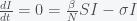(Stationary condition)

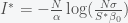
which you can solve to get either or . The point is not a peak but just reflects the fact that there is no epidemic if there are no infections. The other condition gives the peak:

where is the now-famous R naught or initial reproduction number. It is the average number of people infected by a single person since is the infection rate and is the infection disappearance rate, the ratio is a number. The stationary condition gives the herd immunity threshold. When the fraction of reaches then the pandemic will begin to decline.  This is usually expressed as the fraction of those infected and no longer susceptible, . The 70% number you have heard is because is approximately 70% for , the presumed value for Covid-19.

A plateau in the number of new cases per day is an indication that we are at a stationary point in . This is because only a fraction of the total infected are counted as cases and if we assume that the case detection rate is uniform across all , then the number of new cases per day is proportional to . Thus, a plateau in cases means we are at a stationary point in , which we saw above only occurs at a single instance in time. One resolution to this paradox would be if the peak is broad so it looks like a plateau. We can compute how broad the peak is from the second derivative, which gives the rate of change of the rate of change. This is the curvature of the peak. Taking the second derivative of the I equation in the SIR model gives

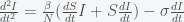
Using and the formula for at the peak, the curvature is

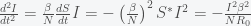
It is negative because at a peak the slope is decreasing. (A hill is easier to climb as you round the top.)  There could be an apparent plateau if the curvature is very small, which is true if is small compared to . However, this would also mean we are already at the herd immunity threshold, which our paper and recent anti-body surveys predict to be unlikely given what we know about .

If a broad peak at the herd immunity threshold does not explain the plateau in new global daily cases then what does? Cochrane’s theory is that depends on .  He postulated that ,where is the initial infectivity rate, but any decreasing function will do. When goes up, goes down. Cochrane attributes this to human behavior but it could also be a result of policy and government mandate. If you plug this into the stationary condition you get

or

and the effective reproduction number   is one.

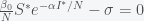
However, this is still only a quasi-stationary state because if is a constant , then 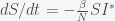will decrease as , which has solution

     (S)

Plugging this into the equation for  gives

which means that is not really plateaued but is decreasing slowly as

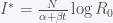
We can establish perfect conditions for a plateau if we work backwards. Suppose again that has plateaued at .  Then, is given by equation (S).  Substituting this into the (Stationary Condition) above then gives or

which means that the global plateau is due to us first reducing to near , which halted the spread locally, and then gradually relaxing pandemic mitigation measures so that is creeping upwards back to it’s original value.

The Covid-19 plateau is both good news and bad news. It is good news because we are not seeing exponential growth of the pandemic. Globally, it is more or less contained. The bad news is that by increasing at a rate of a hundred thousand cases per day, it will take a long time before we reach herd immunity. If we make the naive assumption that we won’t reach herd immunity until 5 billion people are infected then this pandemic could blunder along for days! In other words, the pandemic will keep circling the world forever since over that time span, babies will be born and grow up. Most likely, it will become less virulent and will just join the panoply of diseases we currently live with like the various varieties of the common cold (which are also corona viruses) and the flu.

Exponential growth

The spread of covid-19 and epidemics in general is all about exponential growth. Although, I deal with exponential growth in my work daily, I don’t have an immediate intuitive grasp for what it means in life until I actually think about it. To me I write down functions with the form and treat them as some abstract quantity. In fact, I often just look at differential equations of the form

for which is a solution, where is any constant number, because the derivative of an exponential function is an exponential function. One confusing aspect of discussing exponential growth with lay people is that the above equation is called a linear differential equation and often mathematicians or physicists will simply say the dynamics are linear or even the growth is linear, although what we really mean is that the describing equation is a linear differential equation, which has exponential growth or exponential decay if is negative.

If we let represent time (say days) then is a growth rate. What actually means is that every day , e.g. number of people with covid-19, is increasing by a factor of , which is about 2.718.  Now, while this is the most convenient number for mathematical manipulation, it is definitely not the most convenient number for intuition. A common alternative is to use 2 as the base of the exponent, rather than . This then means that tomorrow you will have double what you have today. I think 2 doesn’t really convey how fast exponential growth is because you say well I start with 1 today and then tomorrow I have 2 and the day after 4 and like the famous Simpson’s episode when Homer is making sure that Bart is a name safe from mockery, goes through the alphabet and says “Aart, Bart, Cart, Dart, Eart, okay Bart is fine,”  you will have to go to day 10 before you get to a thousand fold increase (1024 to be precise), which still doesn’t seem too bad. In fact 30 days later is 2 to the power of 30 or , which is only 10 million or so. But on day 31 you have 20 million and day 32 you have 40 million. It’s growing really fast.

Now, I think exponential growth really hits home if you use 10 as a base because now you simply add a zero for every day: 1, 10, 100, 1000, 10000, 100000. Imagine if your stock was increasing by a factor of 10 every day. Starting from a dollar you would have a million dollars by day 6 and a billion by day 9, be richer than Bill Gates by day 11, and have more money than the entire world by the third week. Now, the only difference between exponential growth with base 2 versus base 10 is the rate of growth. This is where logarithms are very useful  because they are the inverse of an exponential. So, if then (i.e. the log of x in base 2 is 3). Log just gives you the power of an exponential (in that base). So the only difference between using base 2 versus base 10 is the rate of growth. For example , where .  So an exponential process that is doubling every day is increasing by a factor of ten every 3.3 days.

The thing about exponential growth is that most of the action is in the last few days. This is probably the hardest part to comprehend.  So the reason they were putting hospital beds in the convention center in New York weeks ago is because if the number of covid-19 cases is doubling every 5 days then even if you are 100 fold under capacity today, you will be over capacity in 7 doublings or 35 days and the next week you will have twice as many as you can handle.

Flattening the curve means slowing the growth rate. If you can slow the rate of growth by a half then you have 70 days before you get to 7 doublings and max out capacity. If you can make the rate of growth negative then the number of cases will decrease and the epidemic will flame out. There are two ways you can make the growth rate go negative. The first is to use external measures like social distancing and the second is to reach nonlinear saturation, which I’ll discuss in a later post. This is also why social distancing measures seem so extreme and unnecessary because you need to apply it before there is a problem and if it works then those beds in the convention center never get used. It’s a no win situation, if it works then it will seem like an over reaction and if it doesn’t then hospitals will be overwhelmed. Given that 7 billion lives and livelihoods are at stake, it is not a decision to be taken lightly.

 

How to be a scientific dilettante

I have worked in a lot of disparate fields from plasma physics, to nonlinear dynamics, to posture control, to neuroscience, to inflammation, to obesity, to gene transcription, and population genetics. I have had a lot of fun doing this but I definitely do not recommend it as a career path for a young person. I may have gotten away with it but I was really lucky and it certainly carried a cost. First of all, by working in so many fields, I definitely lack the deep knowledge that specialists have. Thus, I don’t always see the big picture and am often a step behind others. Secondly, while I am pretty well cited, my citations are diluted over multiple fields. Thus, while my total H index (number of papers where number of citations exceeds rank) is pretty decent, my H index in each given field is relatively small. I thus do not have much impact in any given area. To be taken seriously as a scientist, one must be a world expert in something. The system is highly nonlinear; being pretty good in a lot of things is much worse than being really good in one thing. There is a threshold for relevance and if you don’t cross it then it is like you don’t exist.

However, if you do want to work in a lot of fields, the worse thing to do is to say, “Hey I really find field X to be interesting so I’m just going to read some books and papers on it and try to do something.” I have reviewed quite a few papers, where some mathematician or physicist has read some popular science book or newspaper article on the topic and then tried to publish a paper on a problem mentioned in the book. I then have to tell them to read up on four decades of previous work first, and then resubmit. The way I have managed to meander through multiple fields is that someone will either contact me directly about some specific question or mention something to me either in a casual setting or at a conference. I could not possibly have made any progress at all if I didn’t have great collaborators who really knew the field and the literature. Still, people constantly ask me if I still work in neuroscience, to which I can only respond “Just because you don’t cite me doesn’t mean I don’t publish!”

 

How the brain constructs the visual world

First there was Carl Sagan, then there was Neil deGrasse Tyson, now there is Michael Buice:

Heritability in twins

Nature Genetics recently published a meta-analysis of virtually all twin studies over the last half century:

Tinca J C Polderman, Beben Benyamin, Christiaan A de Leeuw, Patrick F Sullivan, Arjen van Bochoven, Peter M Visscher & Danielle Posthuma. Meta-analysis of the heritability of human traits based on fifty years of twin studies. Nature Genetics 47,702–709 (2015) doi:10.1038/ng.3285.

One of the authors, Peter Visscher, is perhaps the most influential and innovative thinker in human genetics at this moment and this paper continues his string of insightful results. The paper examined close to eighteen thousand traits in almost three thousand publications, representing fifteen million twins. The main goal was to use all the available data to recompute the heritability estimates for all of these traits. The first thing they found was that the traits were highly skewed towards psychiatric and cognitive phenotypes. People who study heritability are mostly interested in mental function. They then checked to see if there was any publication bias where people only published results with high heritability. They used multiple methods but they basically checked if the predictions of effect size was correlated with sample size and they found none. Their most interesting result, which I will comment on more below was that the average heritability across all traits was 0.488, which means that on average genes and environment contribute equally. However, heritability does vary widely across domains where eye, ear, nose and throat function are most heritable, and social values were least heritable. The largest influence of shared environmental effects was for bodily functions, infections, and social values. Hence, staying healthy depends on your environment, which is why a child who may be stunted in their impoverished village can thrive if moved to Minnesota. It also shows why attitudes on social issues can and do change. Finally, the paper addressed two important technical issues which I will expand on below – 1) previous studies may be underestimating heritability and 2) heritability is mostly additive.

Heritability is the fraction of the variance of a trait due to genetic variance. Here is a link to a previous post explaining heritability although as my colleague Vipul Periwal points out, it is full of words and has no equations. Briefly, there are two types of heritability – broad sense and narrow sense. Broad sense heritability, , is the total genetic variance divided by the phenotypic variance. Narrow sense heritability is the linear or additive genetic variance divided by the phenotypic variance. A linear regression of the standardized trait of the children against the average of the standardized trait of the parents is an estimate of the narrow sense heritability. It captures the linear part while the broad sense heritability includes the linear and nonlinear contributions, which include dominance and gene-gene effects (epistasis). To estimate (narrow-sense) heritability from twins, Polderman et al. used what is called Falconer’s formula and took twice the difference in the correlation of a trait between identical (monozygotic) and fraternal (dizygotic) twins (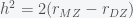). The idea being that the any difference between identical twins must be environmental (nongenetic), while the difference between dyzgotic twins is half genetic and environmental, so the difference between the two is half genetic. They also used another Falconer formula to estimate the shared environmental variance, which is , since this “cancels out” the genetic part. Their paper then boiled down to doing a meta-analysis of and . Meta-analysis is a nuanced topic but it boils down to weighting results from different studies by some estimate of how large the errors are. They used the DerSimonian-Laird random-effects approach, which is implemented in R. The Falconer formulas estimate the narrow sense heritability but many of the previous studies were interested in nonadditive genetic effects as well. Typically, what they did was to use either an ACE (Additive, common environmental, environmental) or an ADE (Additive, dominance, environmental) model. They decided on which model to use by looking at the sign of . If it is positive then they used ACE and if it is negative they used ADE. Polderman et al. showed that this decision algorithm biases the heritability estimate downward.

If the heritability of a trait is mostly additive then you would expect that and they found that this was observed in 69% of the traits. Of the top 20 traits, 8 traits showed nonadditivity and these mostly related to behavioral and cognitive functions. Of these eight, 7 showed that the correlation between monozygotic twins was smaller than twice that of dizygotic twins, which implies that nonlinear genetic effects tend to work against each other. This makes sense to me since it would seem that as you start to accumulate additive variants that increase a phenotype you will start to hit rate limiting effects that will tend to dampen these effects. In other words, it seems plausible that the major nonlinearity in genetics is a saturation effect.

The most striking result was that the average heritability across all of the traits was about 0.5. Is an average value of 0.5 obvious or deep? I honestly do not know. When I told theoretical neuroscientist Fred Hall this result, he thought it was obvious and should be expected from maximum entropy considerations, which would assume that the distribution of would be uniform or at least symmetric about 0.5. This sounds plausible but as I have asserted many times – biology is the result of an exponential amplification of exponentially unlikely events. Traits that are heritable are by definition those that have variation across the population. Some traits, like the number of limbs, have no variance but are entirely genetic. Other traits, like your favourite sports team, are highly variable but not genetic even though there is a high probability that your favourite team will be the same as your parent’s or sibling’s favourite team. Traits that are highly heritable include height and cognitive function. Personality on the other hand, is not highly heritable. One of the biggest puzzles in population genetics is why there is any variability in a trait to start with. Natural selection prunes out variation exponentially fast so if any gene is selected for, it should be fixed very quickly. Hence, it seems equally plausible that traits with high variability would have low heritability. The studied traits were also biased towards mental function and different domains have different heritabilities. Thus, if the traits were sampled differently, the averaged heritability could easily deviate from 0.5. Thus, I think the null hypothesis should be that the value is a coincidence but I’m open to a deeper explanation.

A software tool to investigate these results can be found here. An enterprising student could do some subsampling of the traits to see how likely 0.5 would hold up if our historical interests in phenotypes were different.

Thanks go to Rick Gerkin for suggesting this topic.

Hopfield on the difference between physics and biology

Here is a short essay by theoretical physicist John Hopfield of the Hopfield net and kinetic proofreading fame among many other things (hat tip to Steve Hsu). I think much of the hostility of biologists towards physicists and mathematicians that Hopfield talks about have dissipated over the past 40 years, especially amongst the younger set. In fact these days, a good share of Cell, Science, and Nature papers have some computational or mathematical component. However, the trend is towards brute force big data type analysis rather than the simple elegant conceptual advances that Hopfield was famous for. In the essay, Hopfield gives several anecdotes and summarizes them with pithy words of advice. The one that everyone should really heed and one I try to always follow is “Do your best to make falsifiable predictions. They are the distinction between physics and ‘Just So Stories.’”

Sampling from a probability distribution

When simulating any system with randomness, sampling from a probability distribution is necessary. Usually, you’ll just need to sample from a normal or uniform distribution and thus can use a built-in random number generator. However, for the time when a built-in function does not exist for your distribution, here’s a simple algorithm.

Let’s say you have some probability density function (PDF) on some domain and you want to generate a set of numbers that follows this probability law. This is actually very simple to do although those new to the field may not know how. Generally, any programming language or environment has a built-in random number generator for real numbers (up to machine precision) between 0 and 1. Thus, what you want to do is to find a way to transform these random numbers, which are uniformly distributed on the domain to the random numbers you want. The first thing to notice is that the cumulative distribution function (CDF) for your PDF, is a function that ranges over the interval , since it is a probability. Thus, the algorithm is: 1) generate a random number between o and 1, and 2) plug it into the inverse of . The numbers you get out satisfy your distribution (i.e. ).

If you’re lucky enough to have a closed form expression of the inverse of the CDF then you can just plug the random numbers directly into your function, otherwise you have to do a little more work. If you don’t have a closed form expression for the CDF then you can just solve the equation for . Newton’s method will generally converge very quickly.  You just loop over the command x = x – (P(x)-r)/rho(x) until you reach the tolerance you want. If you don’t have a closed form expression of the CDF then the simplest way is construct the CDF numerically by computing the N dimensional vector , for some discretization parameter such that  .  If the PDF is defined on the entire real line then you’ll have to decide on what you want the minimum and maximum (through ) to be. If the distribution has thin tails, then you just need to go out until the probability is smaller than your desired error tolerance. You then find the index such that is closest to (i.e. in Julia you could use findmin(abs(v[j]-r))) and your random number is .

Here is why the algorithm works. What we are doing is transforming the PDF of , which we can call , to the desired PDF for . The transformation we use is . Thus, or . Now, is just 1 on the interval and is the PDF of as expected. Thus, inverting the CDF for uniform random numbers always gives you a new set of random numbers that satisfies the new PDF. Trivial perhaps, but really useful.

Erratum: 2019-04-05.  It was pointed out to me that my algorithm involving direct summation of the CDF had some errors.  I hope they have now been corrected.

The perils of math pedagogy

It seems that the prevailing wisdom in teaching mathematics is to make abstract concepts as concrete as possible. The thinking is that if math can be related to everyday concepts or pictures then it will be more palatable and understandable. I happen to disagree. I think part of what makes math fun is the abstractness of it. You make up some rules and follow them to their logical conclusions. This is also how I see children play. They like to invent make-believe worlds and then play within them according to the rules of the world.

Usually these attempts at concreteness seem harmless enough but I have recently come up with an example where making things concrete is much more confusing than just teaching a rule. The example is in division with remainders. My third grader was asked to “draw” 7 divided by 2 in terms of items and groups. Her instinct was to draw 2 groups with three balls each with one ball remaining, like this

(x x x)

(x x x)

x

She then was supposed to write this as a mixed number, which looking at the diagram she wrote 3 1/3. When she asked me if this is correct I asked her to multiply this by 2 and see if it gets back 7 and when she got 6 2/3, she was extremely confused as to why she didn’t get the right answer. I tried to explain to her that the way she grouped things, the remainder was in terms of the fraction of the number of groups, which is very unintuitive and almost impossible to explain. It would have been even worse if the example was 8 divided by 3.

I then tried to tell her that a better way to think of division is not to ask how many elements would you get if you divided 7 into 2 groups because this amounts to begging the question (phrase used the correct way), since you need to know the answer before you can do the operation. Rather, what you really want to ask is how many groups would you have if you divided 7 items into groups of size 2 (which is a local rule), whereupon the diagram would be

( x x)

(x x)

(x x)

x

Now if you write down the mixed number you get 3 1/2, which is the correct answer. She then argued vehemently with me that this is not what the teacher taught her, which may or may not be true.

I think even most adults would get confused by this example and maybe working through it would give them a new appreciation of division. However, if you wanted children to learn to divide correctly than teaching them the rule is better. To divide 7 by 2 you find the largest integer that multiplied by 2 fits into 7 and what’s left over is divided by 2. Even better, which introduces and motivates fractions, is that you write 7 divided by 2 as 7/2 and this then becomes 3 1/2. If you learn the rule, you will never end up with 3 1/3.

MCMC for linear models

I’ve been asked in a comment to give a sample of pseudo code for an MCMC algorithm to fit a linear model to some data. See here for the original post on MCMC. With a linear model, you can write down the answer in closed form (see here), so it is a good model to test your algorithm and code.  Here it is in pseudo-Julia code:

#  initial guess for parameters a and b 
a=0
b=0

# construct chi squared, where D is the data vector and x is the vector of the 
# independent quantity

chi = norm(D - (a*x +b))^2;

for n = 1 : total;
# Make random guesses for new normally distributed a and b with mean old a and b 
# and standard deviation asig and bsig

at = a + asig * randn()
bt = b + bsig * randn()

chit = norm(D - (at*x + bt))^2;

# Take ratio of likelihoods, sigma is the data uncertainty
ratio=exp((-chit + chi)/(2*sigma^2));

# Compare the ratio to a uniform random number between 0 and 1, 
# keep new parameters if ratio exceeds random number
if rand() < ratio
a = at;
b = bt;
chi = chit;
end

end

# Keep running until convergence

Symplectic Integrators

Dynamical systems can be divided into two basic types: conservative and dissipative.  In biology, we almost always model dissipative systems and thus if we want to computationally simulate the system almost any numerical solver will do the job (unless the problem is stiff, which I’ll leave to another post). However, when simulating a conservative system, we must take care to conserve the conserved quantities. Here, I will give a very elementary review of symplectic integrators for numerically solving conservative systems.

Michaelis-Menten kinetics

This year is the one hundred anniversary of the Michaelis-Menten equation, which was published in 1913 by German born biochemist Leonor Michaelis and Canadian physician Maud Menten. Menten was one of the first women to obtain a medical degree in Canada and travelled to Berlin to work with Michaelis because women were forbidden from doing research in Canada. After spending a few years in Europe she returned to the US to obtain a PhD from the University of Chicago and spent most of her career at the University of Pittsburgh. Michaelis also eventually moved to the US and had positions at Johns Hopkins University and the Rockefeller University.

The Michaelis-Menten equation is one of the first applications of mathematics to biochemistry and perhaps the most important. These days people, including myself, throw the term Michaelis-Menten around to generally mean any function of the form

although its original derivation was to specify the rate of an enzymatic reaction.  In 1903, it had been discovered that enzymes, which catalyze reactions, work by binding to a substrate. Michaelis took up this line of research and Menten joined him. They focused on the enzyme invertase, which catalyzes the breaking down (i.e. hydrolysis) of the substrate sucrose (i.e. table sugar) into the simple sugars fructose and glucose. They modelled this reaction as

where the enzyme E binds to a substrate S to form a complex ES which releases the enzyme and forms a product P. The goal is to calculate the rate of the appearance of P.

Bayesian model comparison Part 2

In a previous post, I summarized the Bayesian approach to model comparison, which requires the calculation of the Bayes factor between two models. Here I will show one computational approach that I use called thermodynamic integration borrowed from molecular dynamics. Recall, that we need to compute the model likelihood function

    (1)

for each model where is just the parameter dependent likelihood function we used to find the posterior probabilities for the parameters of the model.

The integration over the parameters can be accomplished using the Markov Chain Monte Carlo, which I summarized previously here. We will start by defining the partition function

   (2)

where is an inverse temperature. The derivative of the log of the partition function gives

   (3)

which is equal to the ensemble average of . However, if we assume that the MCMC has reached stationarity then we can replace the ensemble average with a time average .  Integrating (3) over from 0 to 1 gives

From (1) and (2), we see that  , which is what we want to compute  and .

Hence, to perform Bayesian model comparison, we simply run the MCMC for each model at different temperatures (i.e. use as the likelihood in the standard MCMC) and then integrate the log likelihoods over at the end. For a Gaussian likelihood function, changing temperature is equivalent to changing the data “error”. The higher the temperature the larger the presumed error. In practice, I usually run at seven to ten different values of and use a simple trapezoidal rule to integrate over .  I can even do parameter inference and model comparison in the same MCMC run.

Erratum, 2013-5-2013,  I just fixed an error in the final formula

Mass

Since the putative discovery of the Higgs boson this past summer, I have heard and read multiple attempts at explaining what exactly this discovery means. They usually go along the lines of “The Higgs mechanism gives mass to particles by acting like molasses in which particles move around …” More sophisticated accounts will then attempt to explain that the Higgs boson is an excitation in the Higgs field. However, most of the explanations I have encountered assume that most people already know what mass actually is and why particles need to be endowed with it. Given that my seventh grade science teacher didn’t really understand what mass was, I have a feeling that most nonphysicists don’t really have a full appreciation of mass.

To start out, there are actually two kinds of mass. There is inertial mass, which is the resistance to acceleration and is mass that goes into Newton’s second law of   and then there is gravitational mass which is like the “charge” of gravity. The more gravitational mass you have the stronger the gravitational force. Although they didn’t need to be, these two masses happen to be the same.  The equivalence of inertial and gravitational mass is one of the deepest facts of the universe and is the reason that all objects fall at the same rate. Galileo’s apocryphal Leaning Tower of Pisa experiment was a proof that the two masses are the same. You can see this by noting that the gravitational force is given by

Revised SDE and path integral paper

At the MBI last week, I gave a tutorial on using path integrals to compute moments of stochastic differential equations perturbatively.  The slides are the same as the tutorial I gave a few years ago (see here).  I slightly modified the review paper that goes with the talk. I added the explicit computation for the generating functional of the complex Gaussian PDF. The new version can be found here.

Strogatz in the Times

Don’t miss Steve Strogatz’s new series on math in the New York Times. Once again Steve manages to make math both interesting and understandable.

A new strategy for the iterated prisoner’s dilemma game

The game theory world was stunned recently when Bill Press and Freeman Dyson found a new strategy to the iterated prisoner’s dilemma (IPD) game. They show how you can extort an opponent such that the only way they can maximize their payoff is to give you an even higher payoff. The paper, published in PNAS (link here) with a commentary (link here), is so clever and brilliant that I thought it would be worthwhile to write a pedagogical summary for those that are unfamiliar with some of the methods and concepts they use. This paper shows how knowing a little bit of linear algebra can go a really long way to exploring deep ideas.

In the classic prisoner’s dilemma, two prisoner’s are interrogated separately. They have two choices. If they both stay silent (cooperate) they get each get a year in prison. If one confesses (defects) while the other stays silent then the defector is released while the cooperator gets 5 years.  If both defect then they both get 3 years in prison. Hence, even though the highest utility for both of them is to both cooperate, the only logical thing to do is to defect. You can watch this played out on the British television show Golden Balls (see example here). Usually the payout is expressed as a reward so if they both cooperate they both get 3 points, if one defects and the other cooperates then the defector gets 5 points and the cooperator gets zero,  and if they both defect they both get 1  point each. Thus, the combined reward is higher if they both cooperate but since they can’t trust their opponent it is only logical to defect and get at least 1 point.

The prisoner’s dilema changes if you play the game repeatedly because you can now adjust to your opponent and it is not immediately obvious what the best strategy is. Robert Axelrod brought the IPD to public attention when he organized a tournament three decades ago. The results are published in his 1984 book The Evolution of Cooperation.  I first learned about the results in Douglas Hofstader’s Metamagical Themas column in Scientific American in the early 1980s. Axelrod invited a number of game theorists to submit strategies to play IPD and the winner submitted by Anatol Rappaport was called tit-for-tat, where you always cooperate first and then do whatever your opponent does.  Since this was a cooperative strategy with retribution, people have been using this example of how cooperation could evolve ever since those results. Press and Dyson now show that you can win by being nasty. Details of the calculations are below the fold.

Nonlinearity in your wallet

Many human traits like height, IQ, and 50 metre dash times are very close to being normally distributed. The normal distribution (more technically the normal probability density function) or Gaussian function

is the famous bell shaped curve that the histogram of class grades fall on. The shape of the Gaussian is specified by two parameters the mean , which coincides with the peak of the bell, and the standard deviation , which is a measure of how wide the Gaussian is. Let’s take height as an example. There is a 68% chance that any person will be within one standard deviation of the mean and a little more than 95% that you will be within two standard deviations. The tallest one percent are about 2.3 standard deviations from the mean.

The fact that lots of things are normally distributed  is not an accident but a consequence of the central limit theorem (CLT), which may be the most important mathematical law in your life. The theorem says that the probability distribution of a sum of a large number of random things will be normal (i.e. a Gaussian). In the example of height, it suggests that there are perhaps hundreds or thousands of genetic and environmental factors that determine your height, each contributing a little amount. When you add them together you get your height and the distribution is normal.

Now, the one major thing in your life that bucks the normal trend is income and especially wealth distribution. Incomes are extremely non-normal. They have what are called fat tails, meaning that the income of the top earners are much higher than would be expected by a normal distribution. A general rule of thumb called the Pareto Principle is that 20% of the population controls 80% of the wealth. It may even be more skewed these days.

There are many theories as to why income and wealth is distributed the way it is and I won’t go into any of these. What I want to point out is that whatever it is that governs income and wealth, it is definitely nonlinear. The key ingredient in the CLT is that the factors add linearly. If there were some nonlinear combination of the variables then the result need not be normal. It has been argued that some amount of inequality is unavoidable given that we are born with unequal innate traits but the translation of those differences into  income inequality is a social choice to some degree. If we rewarded the contributors to income more linearly, then incomes would be distributed more normally (there would be some inherent skew because incomes must be positive). In some sense, the fact that some sectors of the economy seem to have much higher incomes than other sectors implies a market failure.

Causality and obesity

The standard adage for complex systems as seen in biology and economics is that “correlation does not imply causation.”  The question then is how do you ever prove that something causes something. In the example of obesity, I stated in my New York Times interview that the obesity epidemic was caused by an increase in food availability.  What does that mean? If you strictly follow formal logic then this means that a) an increase in food supply will lead to an increase in obesity (i.e. modus ponens) and b) if there were no obesity epidemic then there would not have been an increase in food availability (i.e. modus tollens). It doesn’t mean that if there were not an increase in food availability then there would be no obesity epidemic.  This is where many people seem to be confused.  The obesity epidemic could have been caused by many things.  Some argue that it was a decline in physical activity. Some say that it is due to some unknown environmental agent. Some believe it is caused by an overconsumption of sugar and high fructose corn syrup. They could all be true and that still doesn’t mean that increased food supply was not a causal factor. Our validated model shows that if you feed the US population the extra food then there will be an  increase in body weight that more than compensates for the observed rise.  We have thus satisfied a) and thus I can claim that the obesity epidemic was caused by an increase in food supply.

Stating that obesity is a complex phenomenon that involves lots of different factors and that there cannot be a simple explanation is not an argument against my assertion. This is what I called hiding behind complexity. Yes, it is true that obesity is complex but that is not an argument for saying that food is not a causal factor. If you want to disprove my assertion then what you need to do is to find a country that does not have an obesity epidemic but did exhibit an increase in food supply that was sufficient to cause it. My plan is to do this by applying our model to other nations as soon as I am able to get ahold of data of body weights over time. This has proved more difficult than I expected. The US should be commended for having good easily accessible data. Another important point to consider is that even if increased food supply caused the obesity epidemic, this does not mean that reducing food supply will reverse it. There could be other effects that maintain it even in the absence of excess food.  As we all know, it’s complicated.