I had a personal situation this past year that kept me from posting much but today I decided to sit down and write something – all by myself without any help from anyone or anything. I could have enlisted the help of Chat GPT or some other large language model (LLM) but I didn’t. These posts generally start out with a foggy idea, which then take on a life of their own. Part of my enjoyment of writing these things is that I really don’t know what they will say until I’m finished. But sometime in the near future I’m pretty sure that WordPress will have a little window where you can type an idea and a LLM will just write the post for you. At first I will resist using it but one day I might not feel well and I’ll try it and like it and eventually all my posts will be created by a generative AI. Soon afterwards, the AI will learn what I like to blog about and how often I do so and it will just start posting on it’s own without my input. Maybe most or all content will be generated by an AI.
These LLMs are created by training a neural network to predict the next word of a sentence, given the previous words, sentences, paragraphs, and essentially everything that has ever been written. The machine is fed some text and produces what it thinks should come next. It then compares its prediction with the actual answer and updates its settings (connection weights) based on some score of how well it did. When fed the entire corpus of human knowledge (or at least what is online), we have all seen how well it can do. As I have speculated previously (see here), this isn’t all too surprising given that the written word is relatively new in our evolutionary history. Thus, humans aren’t really all that good at it and there isn’t all that much variety in what we write. Once an AI has the ability to predict the next word, it doesn’t take much more tinkering to make it generate an entire text. The specific technology that made this generative leap is called a diffusion model, which I may describe in more technical detail in the future. But in the simplest terms, the model finds successive small modifications to transform the initial text (or image or anything) into pure noise. The model can then be run backwards starting from random noise to create text.
When all content is generated by AI, the AI will no longer have any human data on which to further train. Human written culture will then be frozen. The written word will just consist of rehashing of previous thoughts along with random insertions generated by a machine. If the AI starts to train on AI generated text then it could leave human culture entirely. Generally, when these statistical learning machines train on their own generated data they can go unstable and become completely unpredictable. Will the AI be considered conscious by then?
If there are an infinite number of universes or even if a single universe is infinite in extent then each person (or thing) should have an infinite number of doppelgangers, each with a slight variation. The argument is that if the universe is infinite, and most importantly does not repeat itself, then all possible configurations of matter and energy (or bits of stuff) can and will occur. There should be an infinite number of other universe or other parts of our universe that contain another solar system, with a sun and an earth and a you except that maybe one molecule in one of your cells is in a different position or moving at a different velocity. A simple way to think about this is to imagine an infinite black and white TV screen where each pixel can be either black or white. If the screen is nonperiodic then any configuration of pixels can be found somewhere on the screen. This is kind of like how any sequence of numbers can be found in the digits of Pi or an infinite number of monkeys typing will eventually type out Hamlet. This generalizes to changing or time dependent universes where any sequence of flickering pixels will exist somewhere on the screen.
Not all universes are possible if you include any type of universal rule in your universe. Universes that violate the rule are excluded. If the pixels obeyed Newton’s law of motion then arbitrary sequences of pixels could no longer occur because the configuration of pixels in the next moment of time depends on the previous moment. However, we can have all possible worlds if we assume that rules are not universal and can change over different parts of the universe.
Some universes are also excluded if we introduce rational belief. For example, it is possible that there is another universe, like in almost every movie these days, that is like ours but slightly different. However, it is impossible for a purely rational person in a given universe to believe arbitrary things. Rational belief is as strong a constraint on the universe as any law of motion. One cannot believe in the conservation of energy and the Incredible Hulk (who can increase in mass by a factor of a thousand within seconds) at the same time. Energy is not universally conserved in the Marvel Cinematic Universe. (Why these supposedly super-smart scientists in those universes don’t invent a perpetual motion machine is a mystery.) Rationality does not even have to be universal. Just having a single rational person excludes certain universes. Science is impossible in a totally random universe in which nothing is predictable. However, if a person merely believed they were rational but were actually not then any possible universe is again possible.
Ultimately, this boils down to the question of what exactly exists? I for one believe that concepts such as rationality, beauty, and happiness exist as much as matter and energy exists. Thus for me, all possible universes cannot exist. There does not exist a universe where I am happy and there is so much suffering and pain in the world.
In my previous post, I showed that an elevator falling from the surface through the center of the earth due to gravity alone would obey the dynamics of a simple harmonic oscillator. I did not know what would happen if the shaft went through some arbitrary chord through the earth. Rick Gerkin believed that it would take the same amount of time for all chords and it turns out that he is correct. The proof is very simple. Consider any chord (straight path) through the earth. Now take a plane and slice the earth through that chord and the center of the earth. This is always possible because it takes three points to specify a plane. Now looking perpendicular to the plane, you can always rotate the earth such that you see
Let the blue dot represent the elevator on this chord. It will fall towards the midpoint. The total force on the elevator is towards the center of the earth along the vector . From the previous post, we know that the gravitational acceleration is . The force driving the elevator is along the chord and will have a magnitude that is given by times the cosine of the angle between and . But this has magnitude exactly equal to ! Thus, the acceleration of the elevator along the chord is and thus the equation of motion for the elevator is , which will be true for all chords and is the same as what we derived before. Hence, it will take the same amount of time to transit the earth. This is a perfect example of how most problems are solved by conceptualizing them in the right way.
The 2012 remake of the classic film Total Recall features a giant elevator that plunges through the earth from Australia to England. This trip is called the “fall”, which I presume to mean it is propelled by gravity alone in an evacuated tube. The film states that the trip takes 17 minutes (I don’t remember if this is to get to the center of the earth or the other side). It also made some goofy point that the seats flip around in the vehicle when you cross the center because gravity reverses. This makes no sense because when you fall you are weightless and if you are strapped in, what difference does it make what direction you are in. In any case, I was still curious to know if 17 minutes was remotely accurate and the privilege of a physics education is that one is given the tools to calculate the transit time through the earth due to gravity.
The first thing to do is to make an order of magnitude estimate to see if the time is even in the ballpark. For this you only need middle school physics. The gravitational acceleration for a mass at the surface of the earth is . The radius of the earth is 6.371 million metres. Using the formula that distance (which you get by integrating twice over time), you get . Plugging in the numbers gives 1140 seconds or 19 minutes. So it would take 19 minutes to get to the center of the earth if you constantly accelerated at . It would take the same amount of time to get back to the surface. Given that the gravitational acceleration at the surface should be an upper bound, the real transit time should be slower. I don’t know who they consulted but 17 minutes is not too far off.
We can calculate a more accurate time by including the effect of the gravitational force changing as you transit through the earth but this will require calculus. It’s a beautiful calculation so I’ll show it here. Newton’s law for the gravitational force between a point mass m and a point mass M separated by a distance r is
where is the gravitational constant. If we assume that mass M (i.e. earth) is fixed then Newton’s 2nd law of motion for the mass m is given by . The equivalence of inertial mass and gravitational mass means you can divide m from both sides. So, if a mass m were outside of the earth, then it would accelerate towards the earth as
and this number is g when r is the radius of the earth. This is the reason that all objects fall with the same acceleration, apocryphally validated by Galileo on the Tower of Pisa. (It is also the basis of the theory of general relativity).
However, the earth is not a point but an extended ball where each point of the ball exerts a gravitational force on any mass inside or outside of the ball. (Nothing can shield gravity). Thus to compute the force acting on a particle we need to integrate over the contributions of each point inside the earth. Assume that the density of the earth is constant so the mass where is the radius of the earth. The force between two point particles acts in a straight line between the two points. Thus for an extended object like the earth, each point in it will exert a force on a given particle in a different direction. So the calculation involves integrating over vectors. This is greatly simplified because a ball is highly symmetric. Consider the figure below, which is a cross section of the earth sliced down the middle.
The particle/elevator is the red dot, which is located a distance r from the center. (It can be inside or outside of the earth). We will assume that it travels on an axis through the center of the earth. We want to compute the net gravitational force on it from each point in the earth along this central axis. All distances (positive and negative) are measured with respect to the center of the earth. The blue dot is a point inside the earth with coordinates (x,y). There is also the third coordinate coming out of the page but we will not need it. For each blue point on one side of the earth there is another point diametrically opposed to it. The forces exerted by the two blue points on the red point are symmetrical. Their contributions in the y direction are exactly opposite and cancel leaving the net force only along the x axis. In fact there is an entire circle of points with radius y (orthogonal to the page) around the central axis where each point on the circle combines with a partner point on the opposite side to yield a force only along the x axis. Thus to compute the net force on the elevator we just need to integrate the contribution from concentric rings over the volume earth. This reduces an integral over three dimensions to just two.
The magnitude of the force (density) between the blue and red dot is given by
To get the component of the force along the x direction we need to multiple by the cosine of the angle between the central axis and the blue dot, which is
(i.e. ratio of the adjacent to the hypotenuse of the relevant triangle). Now, to capture the contributions for all the pairs on the circle we multiple by the circumference which is . Putting this together gives
The y integral extends from zero to the edge of the earth, which is . (This is R at (the center) and zero at (the poles) as expected). The x integral extends from one pole to the other, hence -R to R. Completing the y integral gives
(*)
The second term comes from the 0 limit of the integral, which is . The square root of a number has positive and negative roots but the denominator here is a distance and thus is always a positive quantity and thus must include the absolute value. The first term of the above integral can be completed straightforwardly (I’ll leave it as an exercise) but the second term must be handled with care because r-x can change sign depending on whether r is greater or less than x. For a particle outside of the earth r-x is always positive and we get
Inside the earth, we must break the integral up into two parts
The first term of (*) integrates to
Using the fact that , we get
(We again need the absolute value sign). For , the particle is outside of the earth) and . Putting everything together gives
Thus, we have explicitly shown that the gravitational force exerted by a uniform ball is equivalent to concentrating all the mass in the center. This formula is true for too.
For we have
Remarkably, the gravitational force on a particle inside the earth is just the force on the surface scaled by the ratio r/R. The equation of motion of the elevator is thus
with
(Recall that the gravitational acceleration at the surface is ). This is the classic equation for a harmonic oscillator with solutions of the form . Thus, a period (i.e. round trip) is given by . Plugging in the numbers gives 5062 seconds or 84 minutes. A transit through the earth once would be half that at 42 minutes and the time to fall to the center of the earth would be 21 minutes, which I find surprisingly close to the back of the envelope estimate.
Now Australia is not exactly antipodal to England so the tube in the movie did not go directly through the center, which would make the calculation much harder. This would be a shorter distance but the gravitational force would be at an angle to the tube so there would be less acceleration and something would need to keep the elevator from rubbing against the walls (wheels or magnetic levitation). I actually don’t know if it would take a shorter or longer time than going through the center. If you calculate it, please let me know.
Inflation, the steady increase of prices and wages, is a nice example of what is called a marginal mode, line attractor, or invariant manifold in dynamical systems. What this means is that the dynamical system governing wages and prices has an equilibrium that is not a single point but rather a line or curve in price and wage space. This is easy to see because if we suddenly one day decided that all prices and wages were to be denominated in some other currency, say Scooby Snacks, nothing should change in the economy. Instead of making 15 dollars an hour, you now make 100 Scooby Snacks an hour and a Starbucks Frappuccino will now cost 25 Scooby Snacks, etc. As long as wages and prices are in balance, it does not matter what they are denominated in. That is why the negative effects of inflation are more subtle than simply having everything cost more. In a true inflationary state your inputs should always balance your outputs but at an ever increasing price. Inflation is bad because it changes how you think about the future and that adjustments to the economy always take time and have costs.
This is why our current situation of price increases does not yet constitute inflation. We are currently experiencing a supply shock that has made goods scarce and thus prices have increased to compensate. Inflation will only take place when businesses start to increase prices and wages in anticipation of future increases. We can show this in a very simple mathematical model. Let P represent some average of all prices and W represent average wages (actually they will represent the logarithm of both quantities but that will not matter for the argument). So in equilibrium P = W. Now suppose there is some supply shock and prices now increase. In order to get back into equilibrium wages should increase so we can write this as
where the dot indicates the first derivative (i.e. rate of change of W is positive if P is greater than W). Similarly, if wages are higher than prices, prices should increase and we have
Now notice that the equilibrium (where there is no change in W or P) is given by W=P but given that there is only one equation and two unknowns, there is no unique solution. W and P can have any value as long as they are the same. W – P = 0 describes a line in W-P space and thus it is called a line attractor. (Mathematicians would call this an invariant manifold because a manifold is a smooth surface and the rate of change does not change (i.e. is invariant) on this surface. Physicists would call this a marginal mode because if you were to solve the eigenvalue equation governing this system, it would have a zero eigenvalue, which means that its eigenvector (called a mode) is on the margin between stable and unstable.) Now if you add the two equations together you get
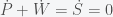
which implies that the rate of change of the sum of P and W, which I call S, is zero. i.e. there is no inflation. Thus if prices and wages respond immediately to changes then there can be no inflation (in this simple model). Now suppose we have instead
The second derivative of W and P respond to differences. This is like having a delay or some momentum. Instead of the rate of S responding to price wage differences, the rate of the momentum of S reacts. Now when we add the two equations together we get
If we integrate this we now get
where C is some nonnegative constant. So in this situation, the rate of change of S is positive and thus S will just keep on increasing forever. Now what is C? Well it is the anticipatory increases in S. If you were lucky enough that C was zero (i.e. no anticipation) then there would be no inflation. Remember that W and P are logarithms so C is the rate of inflation. Interestingly, the way to combat inflation in this simple toy model is to add a first derivative term. This changes the equation to
which is analogous to adding friction to a mechanical system (used differently to what an economist would call friction). The first derivative counters the anticipatory effect of the second derivative. The solution to this equation will return to a state zero inflation (exercise to the reader).
Now of course this model is too simple to actually describe the real economy but I think it gives an intuition to what inflation is and is not.
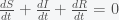
In light of the new omicron variant and breakthrough infections in people who have been vaccinated or previously infected, I was asked to discuss what a model would predict. The simplest model that includes reinfection is an SIRS model, where R, which stands for recovered, can become susceptible again. The equations have the form
I have ignored death due to infection for now. So like the standard SIR model, susceptible, S, have a chance of being infected, I, if they contact I. I then recovers to R but then has a chance to become S again. Starting from an initial condition of S = N and I very small, then S will decrease as I grows.
The first thing to note that the number of people N is conserved in this model (as it should be). You can see this by noting that the sum of the right hand sides of all the equations is zero. Thus and thus the integral is a constant and given that we started with N people then there will remain N people. This will change if we include births and deaths. Given this conservation law, then the dynamics have three possibilities. The first is that it goes to a fixed point meaning that in the long run the numbers of S, I and R will stabilize to some fixed number and remain there forever. The second is that it oscillates so S, I, and R will go up and down. The final one is that the orbit is chaotic meaning that S, I and R will change unpredictably. For these equations, the answer is the first option. Everything will settle to a fixed point.
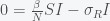
To show this, you first must find an equilibrium or fixed point. You do this by setting all the derivatives to zero and solving the remaining equations. I have always found the fixed point to be the most miraculous state of any dynamical system. In a churning sea where variables move in all directions, there is one place that is perfectly still. The fixed point equations satisfy
There is a trivial fixed point given by S = N and I = R = 0. This is the case of no infection. However, if is large enough then this fixed point is unstable and any amount of I will grow. Assuming I is not zero, we can find another fixed point. Divide I out of the second equation and get
Solving the third equation gives us
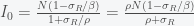
which we can substitute into the first equation to get back the second equation. So to find I, we need to use the conservation condition S + I + R = N which after substituting for S and R gives
which we then back substitute to get
The fact that and must be positive implies is necessary.
The next question is whether this fixed point is stable. Just because a fixed point exists doesn’t mean it is stable. The classic example is a pencil balancing on its tip. Any small perturbation will knock it over. There are many mathematical definitions of stability but they essentially boil down to – does the system return to the equilibrium if you move away from it. The most straightforward way to assess stability is to linearize the system around the fixed point and then see if the linearized system grows or decays (or stays still). We linearize because linear systems are the only types of dynamical systems that can always be solved systematically. Generalizable methods to solve nonlinear systems do not exist. That is why people such as myself can devote a career to studying them. Each system is its own thing. There are standard methods you can try to use but there is no recipe that will always work.
To linearize around a fixed point we first transform to a coordinate system around that fixed point by defining , , , to get
So now s = h = r = 0 is the fixed point. I used lower case h because lower case i is usually . The only nonlinear term is , which we ignore when we linearize. Also by the definition of the fixed point the system then simplifies to
which we can write as a matrix equation
, where and . The trace of the matrix is so the sum of the eigenvalues is negative but the determinant is zero (since the rows sum to zero), and thus the product of the eigenvalues is zero. With a little calculation you can show that this system has two eigenvalues with negative real part and one zero eigenvalue. Thus, the fixed point is not linearly stable but could still be nonlinearly stable, which it probably is since the nonlinear terms are attracting.
That was a lot of tedious math to say that with reinfection, the simplest dynamics will lead to a stable equilibrium where a fixed fraction of the population is infected. The fraction increases with increasing or and decreases with . Thus, as long as the reinfection rate is much smaller than the initial infection rate (which it seems to be), we are headed for a situation where Covid-19 is endemic and will just keep circulating around forever. It may have a seasonal variation like the flu, which is still not well understood and is beyond the simple SIRS equation. If we include death in the equations then there is no longer a nonzero fixed point and the dynamics will just leak slowly towards everyone dying. However, if the death rate is slow enough this will be balanced by births and deaths due to other causes.
Although cryptocurrencies have been mainstream for quite a while, I still think the popular press has not done a great job explaining the details of how they work. There are several ideas behind a cryptocurrency like Bitcoin but the main one is the concept of a cryptographic hash. In simple terms, a hash is a way to transform an input sequence of characters (i.e. a string) into an output string such that it is hard to recreate the input string from the output string. A transformation with this property is called a one-way function. It is a machine where you get an output from an input but you can’t get the input from the output and there does not exist any other machine that can get the input from the output. A hash is a one-way function where the output has a standard form, e.g. 64 characters long. So if each character is a bit, e.g. 0 or 1, then there are different possible hashes. What makes hashes useful are two properties. The first, as mentioned, is that it is a one-way function and the second is that two different inputs do not give the same hash, called collision avoidance. There have been decades of work on figuring out how to do this and institutions like the US National Institutes of Standards and Technology (NIST) actually publish hash standards like SHA-2.
Hashes are an important part of your life. If a company is responsible, then only the hash of your password is stored on their servers, and when you type your password into a website, it goes through the hashing function and the hash is checked against the stored version. That way, if there is security breach, only the hash list is stolen. If the company is very responsible, then your name and all of your information is also only stored in hash form. Part of the problem with past security breaches is that the companies stored actual information instead of hashed information. However, if you use the same password on different websites then the hash would be same if the same standard was used. Some really careful companies will “salt” your password by adding a random string to it (that is hopefullly stored separately) before hashing. Or they will rehash your hash with salt. If you had a perfect hash, then the only way to break it would be to guess different inputs and see if it matches the desired output. The so-called complex math problem that Bitcoin solves before validating a transaction (and getting a reward) is finding a hash with a certain property but more on this later.
Now, one of the problems with hashing is that you need to deal with inputs of various sizes but you want the output to have a single uniform size. So even though a hash could have enough information capacity (i.e. entropy) to encode all of the world’s information ten times over, it is computationally inconvenient to just feed the complete text of Hamlet directly into a single one-way function. This is where the concept of a Merkle tree becomes important. You start with some one-way function that takes inputs of some fixed length and it scrambles the characters in some way that is not easily reversible. If the input string is too short then you just add extra characters (called padding) but if it is too long you need to do something else. The way a Merkle tree works is to break the text into chunks of uniform size. It then hashes the first chunk, adds that to the next chunk, hash the result and repeat until you have included all the chunks. This repeated recursive hashing is the secret sauce of crypto-currencies.
Bitcoin tried to create a completely decentralized digital currency that could be secure and trusted. For a regular currency like the US dollar, the thing you are most concerned about is that the dollar you receive is not counterfeit. The way that problem is solved is to make the manufacturing process of dollar bills very difficult to reproduce. So the dollar uses special paper with special marks and threads and special fonts and special ink. There are laws against making photocopiers with a higher resolution than the smallest print on a US bill to safeguard against counterfeiting. A problem with digital currencies is that you need to prevent double spending. The way this is historically solved is to have all transactions validated by a central authority.
Bitcoin solves these problems in a decentralized system by using a public ledger, called a blockchain that is time stamped, immutable and verifiable. The block chain keeps track of every Bitcoin transaction. So if you wanted to transfer one Bitcoin to someone else then the blockchain would show that your private Bitcoin ID has one less Bitcoin and the ID of the person you transferred to would have one extra Bitcoin. It is called a blockchain because each transaction (or set of transactions) is recorded into a block, the blocks are sequential, and each block contains a hash of the previous block. To validate a transaction you would need to validate each transaction leading up to the last block to validate that the hash on each block is correct. Thus the blockchain is a Merkle tree ledger where each entry is time stamped, immutable, and verifiable. If you want to change a block you need to change all the blocks before it.
However, the blockchain is not decentralized on its own. How do you prevent two blocks with two different hashes? The way to achieve that goal is to make the hash used in each block have a special form that is hard to find. This underlies the concept of “proof of work”. Bitcoin uses a hash called SHA-256 which consists of a hexadecimal string of 64 characters (i.e. a base 16 number, usually with characters consisting of the digits 0-9 plus letters a-f). Before each block gets added to the chain, it must have a hash that has a set number of zeros at the front. In order to do this, you need to add some random numbers to the block or rearrange it so that the hash changes. This is what Bitcoin miners do. They try different variations of the block until they get a hash that has a certain number of zeros in front and then they race to see who gets it first. The more zeros you need the more guesses you need and thus the harder the computation. If it’s just one zero then one in 16 hashes will have that property and thus on average 16 tries will get you the hash and the right to add to the blockchain. Each time you require an additional zero, the number of possibilities decreases by a factor of 16 so it is 16 times harder to find one. Bitcoin wants to keep the computation time around 15 minutes so as computation speed increases it just adds another zero. The result is an endless arms race. The faster the computers get the harder the hash is to find. The incentive for miners to be fast is that they get some Bitcoins if they are successful in being the first to find a desired hash and earning the right to add a block to the chain.
The actual details for how this works is pretty complicated. All the miners (or Bitcoin nodes) must validate that the proposed block is correct and then they all must agree to add that to the chain. The way it works in a decentralized way is that the code is written so that a node will follow the longest chain. In principle, this is secure because a dishonest miner who wants to change a previous block must change all blocks following it and thus as long as there are more honest miners than dishonest ones, the dishonest ones can never catch up. However, there are issues when two miners simultaneously come up with a hash and they can’t agree on which to follow. This is called a fork and has happened at least once I believe. This gets fixed eventually because honest miners will adopt the longest chain and the chain with the most adherents will grow the fastest. However, in reality there are only a small number of miners that regularly add to the chain so we’re at a point now where a dishonest actor could possibly dominate the honest ones and change the blockchain. Proof of work is also not the only way to add to a blockchain. There are several creative ideas to make it less wasteful or even make all that computation useful and I may write about them in the future. I’m somewhat skeptical about the long term viability of Bitcoin per se but I think the concepts of the blockchain are revolutionary and here to stay.
2021-06-21: some typos fixed and clarifying text added.
Interesting article in the New York Times today about how people to this day still do not know how magician David Berglass did his “Any Card At Any Number” trick. In this trick, a magician asks a person or two to name a card (e.g. Queen of Hearts) and a number (e.g. 37) and then in a variety of ways produce a deck where that card appears at that order in the deck. The supposed standard way to do the trick is for the magician to manipulate the cards in some way but Berglass does his trick by never touching the cards. He can even do the trick impromptu when you visit him by leading you to a deck of cards somewhere in the room or from his pocket that has the card in the correct place. Now, I have no idea how he or anyone does this trick but one way to do the trick is to use “full enumeration”, i.e. hide decks where every possibility is accounted for and then the trick is to remember which deck has that choice. So then the question is how many decks would you need? Well the minimal number of decks is 52 because a particular card could be in one of 52 positions. But how many more decks would you need? The answer is zero. 52 is all you need because for any particular arrangement of cards, each card is in one position. Then all you do is rotate all the cards by one, so the card in the first position is now in the second position for deck 2 and 52 moves to 1 and so on. What the magician can do is to then hide 52 decks and remember the order of each deck. In the article he picked the reporter’s card to within 1 but claimed he may only be able to do it to within 2. That means he’s hiding the decks in groups of 3 and 4 say and then points you to that location and lets you choose which deck.
Since, the discovery of exoplanets nearly 3 decades ago most astronomers, at least the public facing ones, seem to agree that it is just a matter of time before they find signs of life such as the presence of volatile gases in the atmosphere associated with life like methane or oxygen. I’m an agnostic on the existence of life outside of earth because we don’t have any clue as to how easy or hard it is for life to form. To me, it is equally possible that the visible universe is teeming with life or that we are alone. We simply do not know.
But what would happen if we find life on another planet. How would that change our expected probability for life in the universe? MIT astronomer Sara Seager once made an offhand remark in a podcast that finding another planet with life would make it very likely there were many more. But is this true? Does the existence of another planet with life mean a dramatic increase in the probability of life in the universe. We can find out by doing the calculation.
Suppose you believe that the probability of life on a planet is (i.e. fraction of planets with life) and this probability is uniform across the universe. Then if you search planets, the probability for the number of planets with life you will find is given by a Binomial distribution. The probability that there are planets is given by the expression , where is a factor (the binomial coefficient) such that the sum of from one to is 1. By Bayes Theorem, the posterior probability for (yes, that would be the probability of a probability) is given by
where . As expected, the posterior depends strongly on the prior. A convenient way to express the prior probability is to use a Beta distribution
(*)
where is again a normalization constant (the Beta function). The mean of a beta distribution is given by and the variance, which is a measure of uncertainty, is given by . The posterior distribution for after observing planets with life out of will be
where is a normalization factor. This is again a Beta distribution. The Beta distribution is called the conjugate prior for the Binomial because it’s form is preserved in the posterior.
Applying Bayes theorem in equation (*), we see that the mean and variance of the posterior become and , respectively. Now let’s consider how our priors have updated. Suppose our prior was , which gives a uniform distribution for on the range 0 to 1. It has a mean of 1/2 and a variance of 1/12. If we find one planet with life after checking 10,000 planets then our expected becomes 2/10002 with variance . The observation of a single planet has greatly reduced our uncertainty and we now expect about 1 in 5000 planets to have life. Now what happens if we find no planets. Then, our expected only drops to 1 in 10000 and the variance is about the same. So, the difference between finding a planet versus not finding a planet only halves our posterior if we had no prior bias. But suppose we are really skeptical and have a prior with and so our expected probability is zero with zero variance. The observation of a single planet increases our posterior to 1 in 10001 with about the same small variance. However, if we find a single planet out of much fewer observations like 100, then our expected probability for life would be even higher but with more uncertainty. In any case, Sara Seager’s intuition is correct – finding a planet would be a game breaker and not finding one shouldn’t really discourage us that much.
For the past four years, I have been unable to post with any regularity. I have dozens of unfinished posts sitting in my drafts folder. I would start with a thought but then get stuck, which had previously been somewhat unusual for me. Now on this first hopeful day I have had for the past four trying years, I am hoping I will be able to post more regularly again.
Prior to what I will now call the Dark Years, I viewed all of history through an economic lens. I bought into the standard twentieth century leftist academic notion that wars, conflicts, social movements, and cultural changes all have economic underpinnings. But I now realize that this is incorrect or at least incomplete. Economics surely plays a role in history but what really motivates people are stories and stories are what led us to the Dark Years and perhaps to get us out.
Trump became president because he had a story. The insurrectionists who stormed the Capitol had a story. It was a bat shit crazy lunatic story but it was still a story. However, the tragic thing about the Trump story (or rather my story of the Trump story) is that it is an unintentional algorithmically generated story. Trump is the first (and probably not last) purely machine learning president (although he may not consciously know that). Everything he did was based on the feedback he got from his Twitter Tweets and Fox News. His objective function was attention and he would do anything to get more attention. Of the many lessons we will take from the Dark Years, one should be how machine learning and artificial intelligence can go so very wrong. Trump’s candidacy and presidency was based on a simple stochastic greedy algorithm for attention. He would Tweet randomly and follow up on the Tweets that got the most attention. However, the problem with a greedy algorithm (and yes that is a technical term that just happens to coincidentally be apropos) is that once you follow a path it is hard to make a correction. I actually believe that if some of Trump’s earliest Tweets from say 2009-2014 had gone another way, he could have been a different president. Unfortunately, one of his early Tweet themes that garnered a lot of attention was on the Obama birther conspiracy. This lit up both racist Twitter and a counter reaction from liberal Twitter, which led him further to the right and ultimately to the presidency. His innate prejudices biased him towards a darker path and he did go completely unhinged after he lost the election but he is unprincipled and immature enough to change course if he had enough incentive to do so.
Unlike standard machine learning for categorizing images or translating languages, the Trump machine learning algorithm changes the data. Every Tweet alters the audience and the reinforcing feedback between Trump’s Tweets and its reaction can manufacture discontent out of nothing. A person could just happen to follow Trump because they like The Apprentice reality show Trump starred in and be having a bad day because they missed the bus or didn’t get a promotion. Then they see a Trump Tweet, follow the link in it and suddenly they find a conspiracy theory that “explains” why they feel disenchanted. They retweet and this repeats. Trump sees what goes viral and Tweets more on the same topic. This positive feedback loop just generated something out of random noise. The conspiracy theorizing then starts it’s own reinforcing feedback loop and before you know it we have a crazed mob bashing down the Capitol doors with impunity.
Ironically Trump, who craved and idolized power, failed to understand the power he actually had and if he had a better algorithm (or just any strategy at all), he would have been reelected in a landslide. Even before he was elected, Trump had already won over the far right and he could have started moving in any direction he wished. He could have moderated on many issues. Even maintaining his absolute ignorance of how govening actually works, he could have had his wall by having it be part of actual infrastructure and immigration bills. He could have directly addressed the COVID-19 pandemic. He would not have lost much of his base and would have easily gained an extra 10 million votes. Maybe, just maybe if liberal Twitter simply ignored the early incendiary Tweets and only responded to the more productive ones, they could have moved him a bit too. Positive reinforcement is how they train animals after all.
Now that Trump has shown how machine learning can win a presidency, it is only a matter of time before someone harnesses it again and more effectively. I just hope that person is not another narcissistic sociopath.
On some rare days when the sun is shining and I’m enjoying a well made kouign-amann (my favourite comes from b.patisserie in San Francisco but Patisserie Poupon in Baltimore will do the trick), I find a brief respite from my usual depressed state and take delight, if only for a brief moment, in the fact that mathematics completely resolved Zeno’s paradox. To me, it is the quintessential example of how mathematics can fully solve a philosophical problem and it is a shame that most people still don’t seem to know or understand this monumental fact. Although there are probably thousands of articles on Zeno’s paradox on the internet (I haven’t bothered to actually check), I feel like visiting it again today even without a kouign-amann in hand.
I don’t know what the original statement of the paradox is but they all involve motion from one location to another like walking towards a wall or throwing a javelin at a target. When you walk towards a wall, you must first cross half the distance, then half the remaining distance, and so on forever. The paradox is thus: How then can you ever reach the wall, or a javelin reach its target, if it must traverse an infinite number of intervals? This paradox is completely resolved by the concept of the mathematical limit, which Newton used to invent calculus in the seventeenth century. I think understanding the limit is the greatest leap a mathematics student must take in all of mathematics. It took mathematicians two centuries to fully formalize it although we don’t need most of that machinery to resolve Zeno’s paradox. In fact, you need no more than middle school math to solve one of history’s most famous problems.
The solution to Zeno’s paradox stems from the fact that if you move at constant velocity then it takes half the time to cross half the distance and the sum of an infinite number of intervals that are half as long as the previous interval adds up to a finite number. That’s it! It doesn’t take forever to get anywhere because you are adding an infinite number of things that get infinitesimally smaller. The sum of a bunch of terms is called a series and the sum of an infinite number of terms is called an infinite series. The beautiful thing is that we can compute this particular infinite series exactly, which is not true of all series.
Expressed mathematically, the total time it takes for an object traveling at constant velocity to reach its target is
which can be rewritten as
where is the distance and is the velocity. This infinite series is technically called a geometric series because the ratio of two subsequent terms in the series is always the same. The terms are related geometrically like the volumes of n-dimensional cubes when you have halve the length of the sides (e.g. 1-cube (line and volume is length), 2-cube (square and volume is area), 3-cube (good old cube and volume), 4-cube ( hypercube and hypervolume), etc) .
For simplicity we can take . So to compute the time it takes to travel the distance, we must compute:
To solve this sum, the first thing is to notice that we can factor out and obtain
The quantity inside the bracket is just the original series plus 1, i.e.
and thus we can substitute this back into the original expression for and obtain
Now, we simply solve for and I’ll actually go over all the algebraic steps. First multiply both sides by 2 and get
Now, subtract from both sides and you get the beautiful answer that . We then have the amazing fact that
I never get tired of this. In fact this generalizes to any geometric series
for any that is less than 1. The more compact way to express this is
Now, notice that in this formula if you set , you get , which is infinity. Since for any , this tells you that if you try to add up an infinite number of ones, you’ll get infinity. Now if you set you’ll get a negative number. Does this mean that the sum of an infinite number of positive numbers greater than 1 is a negative number? Well no because the series is only defined for , which is called the domain of convergence. If you go outside of the domain, you can still get an answer but it won’t be the answer to your question. You always need to be careful when you add and subtract infinite quantities. Depending on the circumstance it may or may not give you sensible answers. Getting that right is what math is all about.
Among the myriad of problems we are having with the COVID-19 pandemic, faster testing is one we could actually improve. The standard test for the presence of SARS-CoV-2 virus uses PCR (polymerase chain reaction), which amplifies targeted viral RNA. It is accurate (high specificity) but requires relatively expensive equipment and reagents that are currently in short supply. There are reports of wait times of over a week, which renders a test useless for contact tracing.
An alternative to PCR is an antigen test that tests for the presence of protein fragments associated with COVID-19. These tests can in principle be very cheap and fast, and could even be administered on paper strips. They are generally much more unreliable than PCR and thus have not been widely adopted. However, as I show below by applying the test multiple times, the noise can be suppressed and a poor test can be made arbitrarily good.
The performance of binary tests are usually gauged by two quantities – sensitivity and specificity. Sensitivity is the probability that you test positive (i.e are infected) given that you actually are positive (true positive rate). Specificity is the probability that you test negative if you actually are negative (true negative rate). For a pandemic, sensitivity is more important than specificity because missing someone who is infected means you could put lots of people at risk while a false positive just means the person falsely testing positive is inconvenienced (provided they cooperatively self-isolate). Current PCR tests have very high specificity but relatively low sensitivity (as low as 0.7) and since we don’t have enough capability to retest, a lot of tested infected people could be escaping detection.
The way to make any test have arbitrarily high sensitivity and specificity is to apply it multiple times and take some sort of average. However, you want to do this with the fewest number of applications. Suppose we administer tests on the same subject, the probability of getting more than positive tests if the person is positive is , where is the cumulative distribution function of the Binomial distribution (i.e. probability that the number of Binomial distributed events is less than or equal to ). If the person is negative then the probability of or fewer positives is . We thus want to find the minimal given a desired sensitivity and specificity, and . This means that we need to solve the constrained optimization problem: find the minimal under the constraint that , and . decreases and increases with increasing and vice versa for . We can easily solve this problem by sequentially increasing and scanning through until the two constraints are met. I’ve included the Julia code to do this below. For example, starting with a test with sensitivity .7 and specificity 1 (like a PCR test), you can create a new test with greater than .95 sensitivity and specificity, by administering the test 3 times and looking for a single positive test. However, if the specificity drops to .7 then you would need to find more than 8 positives out of 17 applications to be 95% sure you have COVID-19.
using Distributions
function Q(k,n,q)
d = Binomial(n,q)
return 1 – cdf(d,k)
end
function R(k,n,r)
d = Binomial(n,1-r)
return cdf(d,k)
end
function optimizetest(q,r,qp=.95,rp=.95)
nout = 0
kout = 0
for n in 1:100
for k in 0:n-1
println(R(k,n,r),” “,Q(k,n,q))
if R(k,n,r) >= rp && Q(k,n,q) >= qp
kout=k
nout=n
break
end
end
if nout > 0
break
end
end
Here are my slides for my recent COVID-19 talk at the Centre for Applied Mathematics in BioScience and Medicine (CAMBAM). It’s an updated version of the one I gave to the FDA.
Right now there are hundreds if not thousands of Covid-19 models floating out there. Some are better than others and some have much more influence than others and the ones that have the most influence are not necessarily the best. There must be a better way of doing this. The world’s greatest minds convened in Los Alamos in WWII and built two atomic bombs. Metaphors get thrown around with reckless abandon but if there ever was a time for a Manhattan project, we need one now. Currently, the world’s scientific community has mobilized to come up with models to predict the spread and effectiveness of mitigation efforts, to produce new therapeutics and to develop new vaccines. But this is mostly going on independently.
Would it be better if we were to coordinate all of this activity. Right now at the NIH, there is an intense effort to compile all the research that is being done in the NIH Intramural Program and to develop a system where people can share reagents and materials. There are other coordination efforts going on worldwide as well. This website contains a list of open source computational resources. This link gives a list of data scientists who have banded together. But I think we need a world wide plan if we are ever to return to normal activity. Even if some nation has eliminated the virus completely within its borders there is always a chance of reinfection from outside.
In terms of models, they seem to have very weak predictive ability. This is probably because they are all over fit. We don’t really understand all the mechanisms of SARS-CoV-2 propagation. The case or death curves are pretty simple and as Von Neumann or Ulam or someone once said, “give me 4 parameters and I can fit an elephant, give me 5 and I can make it’s tail wiggle.” Almost any model can fit the curve but to make a projection into the future, you need to get the dynamics correct and this I claim, we have not done. What I am thinking of proposing is to have the equivalent of FDA approval for predictive models. However, instead of a binary decision of approval non-approval, people could submit there models for a predictive score based on some cross validation scheme or prediction on a held out set. You could also submit as many times as you wish to have your score updated. We could then pool all the models and produce a global Bayesian model averaged prediction and see if that does better. Let me know if you wish to participate or ideas on how to do this better.
First draft of our paper can be downloaded from this link. I’ll post more details about it later.
Global prediction of unreported SARS-CoV2 infection from observed COVID-19 cases
Carson C. Chow 1*, Joshua C. Chang 2,3, Richard C. Gerkin 4*, Shashaank Vattikuti 1*
1Mathematical Biology Section, LBM, NIDDK, National Institutes of Health2Epidemiology and Biostatistics Section, Rehabilitation Medicine, Clinical Center, National Institutes of Health 3 mederrata 4 School of Life Sciences, Arizona State University
Summary: Estimation of infectiousness and fatality of the SARS-CoV-2 virus in the COVID-19 global pandemic is complicated by ascertainment bias resulting from incomplete and non-representative samples of infected individuals. We developed a strategy for overcoming this bias to obtain more plausible estimates of the true values of key epidemiological variables. We fit mechanistic Bayesian latent-variable SIR models to confirmed COVID-19 cases, deaths, and recoveries, for all regions (countries and US states) independently. Bayesian averaging over models, we find that the raw infection incidence rate underestimates the true rate by a factor, the case ascertainment ratio CARt that depends upon region and time. At the regional onset of COVID-19, the predicted global median was 13 infections unreported for each case confirmed (CARt = 0.07 C.I. (0.02, 0.4)). As the infection spread, the median CARt rose to 9 unreported cases for every one diagnosed as of April 15, 2020 (CARt = 0.1 C.I. (0.02, 0.5)). We also estimate that the median global initial reproduction number R0 is 3.3 (C.I (1.5, 8.3)) and the total infection fatality rate near the onset is 0.17% (C.I. (0.05%, 0.9%)). However the time-dependent reproduction number Rt and infection fatality rate as of April 15 were 1.2 (C.I. (0.6, 2.5)) and 0.8% (C.I. (0.2%,4%)), respectively. We find that there is great variability between country- and state-level values. Our estimates are consistent with recent serological estimates of cumulative infections for the state of New York, but inconsistent with claims that very large fractions of the population have already been infected in most other regions. For most regions, our estimates imply a great deal of uncertainty about the current state and trajectory of the epidemic.
The spread of covid-19 and epidemics in general is all about exponential growth. Although, I deal with exponential growth in my work daily, I don’t have an immediate intuitive grasp for what it means in life until I actually think about it. To me I write down functions with the form and treat them as some abstract quantity. In fact, I often just look at differential equations of the form
for which is a solution, where is any constant number, because the derivative of an exponential function is an exponential function. One confusing aspect of discussing exponential growth with lay people is that the above equation is called a linear differential equation and often mathematicians or physicists will simply say the dynamics are linear or even the growth is linear, although what we really mean is that the describing equation is a linear differential equation, which has exponential growth or exponential decay if is negative.
If we let represent time (say days) then is a growth rate. What actually means is that every day , e.g. number of people with covid-19, is increasing by a factor of , which is about 2.718. Now, while this is the most convenient number for mathematical manipulation, it is definitely not the most convenient number for intuition. A common alternative is to use 2 as the base of the exponent, rather than . This then means that tomorrow you will have double what you have today. I think 2 doesn’t really convey how fast exponential growth is because you say well I start with 1 today and then tomorrow I have 2 and the day after 4 and like the famous Simpson’s episode when Homer is making sure that Bart is a name safe from mockery, goes through the alphabet and says “Aart, Bart, Cart, Dart, Eart, okay Bart is fine,” you will have to go to day 10 before you get to a thousand fold increase (1024 to be precise), which still doesn’t seem too bad. In fact 30 days later is 2 to the power of 30 or , which is only 10 million or so. But on day 31 you have 20 million and day 32 you have 40 million. It’s growing really fast.
Now, I think exponential growth really hits home if you use 10 as a base because now you simply add a zero for every day: 1, 10, 100, 1000, 10000, 100000. Imagine if your stock was increasing by a factor of 10 every day. Starting from a dollar you would have a million dollars by day 6 and a billion by day 9, be richer than Bill Gates by day 11, and have more money than the entire world by the third week. Now, the only difference between exponential growth with base 2 versus base 10 is the rate of growth. This is where logarithms are very useful because they are the inverse of an exponential. So, if then (i.e. the log of x in base 2 is 3). Log just gives you the power of an exponential (in that base). So the only difference between using base 2 versus base 10 is the rate of growth. For example , where . So an exponential process that is doubling every day is increasing by a factor of ten every 3.3 days.
The thing about exponential growth is that most of the action is in the last few days. This is probably the hardest part to comprehend. So the reason they were putting hospital beds in the convention center in New York weeks ago is because if the number of covid-19 cases is doubling every 5 days then even if you are 100 fold under capacity today, you will be over capacity in 7 doublings or 35 days and the next week you will have twice as many as you can handle.
Flattening the curve means slowing the growth rate. If you can slow the rate of growth by a half then you have 70 days before you get to 7 doublings and max out capacity. If you can make the rate of growth negative then the number of cases will decrease and the epidemic will flame out. There are two ways you can make the growth rate go negative. The first is to use external measures like social distancing and the second is to reach nonlinear saturation, which I’ll discuss in a later post. This is also why social distancing measures seem so extreme and unnecessary because you need to apply it before there is a problem and if it works then those beds in the convention center never get used. It’s a no win situation, if it works then it will seem like an over reaction and if it doesn’t then hospitals will be overwhelmed. Given that 7 billion lives and livelihoods are at stake, it is not a decision to be taken lightly.
I have officially thrown my hat into the ring and joined the throngs of would-be Covid-19 modelers to try to estimate (I deliberately do not use predict) the progression of the pandemic. I will pull rank and declare that I kind of do this type of thing for a living. What I (and my colleagues whom I have conscripted) are trying to do is to estimate the fraction of the population that has the SARS-CoV-2 virus but has not been identified as such. This was the goal of the Lourenco et al. paper I wrote about previously that pulled me into this pit of despair. I argued that fitting to deaths alone, which is what they do, is insufficient for constraining the model and thus it has no predictive ability. What I’m doing now is seeing whether it is possible to do the job if you fit not only deaths but also the number of cases reported and cases recovered. You then have a latent variable model where the observed variables are cases, cases that die, and cases that recover, and the latent variables are the infected that are not identified and the susceptible population. Our plan is to test a wide range of models with various degrees of detail and complexity and use Bayesian Model Comparison to see which does a better job. We will apply the analysis to global data. We’re getting numbers now but I’m not sure I trust them yet so I’ll keep computing for a few more days. The full goal is to quantify the uncertainty in a principled way.
Here is my response to the paper from Oxford (Lourenco et al.) arguing that novel coronavirus infection may already be widespread in the UK and Italy. The result is based on fitting a disease spreading model, called an SIR model, to the cumulative number of deaths. SIR models usually consist of ordinary differential equations (ODEs) for the fraction of people in a given population who are susceptible to the infectious agent (S), the number infected (I), and the number recovered (R). There is one other state in the model, which is the fraction who die from the disease (D). The SIR model considers transitions between these states. In the case of ODEs, the states are treated as continuous quantities, which is not a bad approximation for a large population, and each equation in the model describes the rate of change of a state (hence differential equation). There are parameters in the model governing the rate of different interactions in each equation, for example there is a parameter for the rate of increase in S whenever an S interacts with an I, and then there is a rate of loss of an I, which transitions into either R or D. The Oxford group model D somewhat differently. Instead of a transition from I into D they consider that a fraction of (1-S) will die with some delay between time of infection and death.
They estimate the model parameters by fitting the model to the cumulative number of deaths. They did this instead of fitting directly to I because that is unreliable as many people who have Covid-19 have not been tested. They also only fit to the first 15 days from the first recorded death since they want to model what happens before social distancing was implemented. They find that the model is consistent with a scenario where the probability that an infected person gets severe enough to be flagged is low and thus the disease is much more wide spread than expected. I redid the analysis without assuming that the parameters need to have particular values (called priors in Bayesian inference and machine learning) and showed that a wide range of parameters will fit the data. This is because the model is under-constrained by death data alone so even unrealistic parameters can work. To be fair, the authors only proposed that this is a possibility and thus the population should be tested for anti-bodies to the coronavirus (SARS-CoV-2) to see if indeed there may already be herd immunity in place. However, the press has run with the result and that is why I think it is important to examine the result more closely.
We live in an age of fear and yet life (in the US at least) is the safest it has ever been. Megan McArdle blames coddling parents and the media in a Washington Post column. She argues that cars and swimming pools are much more dangerous than school shootings and kidnappings yet we mostly ignore the former and obsess about the latter. However, to me dying from an improbable event is just so much more tragic than dying from an expected one. I would be much less despondent meeting St. Peter at the Pearly Gates if I happened to expire from cancer or heart disease than if I were to be hit by an asteroid while weeding my garden. We are so scared now because we have never been safer. We would fear terrorist attacks less if they were more frequent. This is the reason that I would never want a major increase in lifespan. I most certainly would like to last long enough to see my children become independent but anything beyond that is bonus time. Nothing could be worse to me than immortality. The pain of any tragedy would be unbearable. Life would consist of an endless accumulation of sad memories. The way out is to forget but that to me is no different from death. What would be the point of living forever if you were to erase much of it. What would a life be if you forgot the people and things that you loved? To me that is no life at all.

 . From the previous post, we know that the gravitational acceleration is
  . The force driving the elevator is along the chord and will have a magnitude that is given by
  and
and  and thus the equation of motion for the elevator is
  , which will be true for all chords and is the same as what we derived before. Hence, it will take the same amount of time to transit the earth. This is a perfect example of how most problems are solved by conceptualizing them in the right way.
 . The radius of the earth is 6.371 million metres. Using the formula that distance
  (which you get by integrating twice over time), you get
  . Plugging in the numbers gives 1140 seconds or 19 minutes. So it would take 19 minutes to get to the center of the earth if you constantly accelerated at
  . It would take the same amount of time to get back to the surface. Given that the gravitational acceleration at the surface should be an upper bound, the real transit time should be slower. I don’t know who they consulted but 17 minutes is not too far off.
 is the gravitational constant. If we assume that mass M (i.e. earth) is fixed then Newton’s 2nd law of motion for the mass m is given by
  . The equivalence of inertial mass and gravitational mass means you can divide m from both sides. So, if a mass m were outside of the earth, then it would accelerate towards the earth as
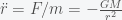
 is constant so the mass
  where
where  is the radius of the earth. The force between two point particles acts in a straight line between the two points. Thus for an extended object like the earth, each point in it will exert a force on a given particle in a different direction. So the calculation involves integrating over vectors. This is greatly simplified because a ball is highly symmetric. Consider the figure below, which is a cross section of the earth sliced down the middle.
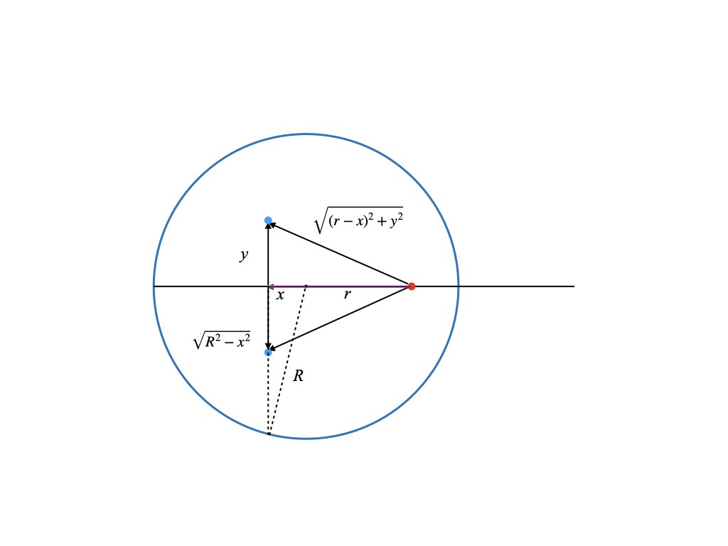


 . Putting this together gives
 . (This is R at
  (the center) and zero at
  (the poles) as expected). The x integral extends from one pole to the other, hence -R to R. Completing the y integral gives
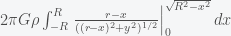
![= 2\pi G\rho \int_{-R}^{R}\left[ \frac{r-x}{((r-x)^2+R^2-x^2)^{1/2}} - \frac{r-x}{|r-x|} \right]dx](https://s0.wp.com/latex.php?latex=%3D+2%5Cpi+G%5Crho+%5Cint_%7B-R%7D%5E%7BR%7D%5Cleft%5B+%5Cfrac%7Br-x%7D%7B%28%28r-x%29%5E2%2BR%5E2-x%5E2%29%5E%7B1%2F2%7D%7D+-+%5Cfrac%7Br-x%7D%7B%7Cr-x%7C%7D+%5Cright%5Ddx&bg=f5f6f7&fg=444444&s=0&c=20201002) (*)
(*) . The square root of a number has positive and negative roots but the denominator here is a distance and thus is always a positive quantity and thus must include the absolute value. The first term of the above integral can be completed straightforwardly (I’ll leave it as an exercise) but the second term must be handled with care because r-x can change sign depending on whether r is greater or less than x. For a particle outside of the earth r-x is always positive and we get

![\left[ \frac{(r^2-2rx+R^2)^{1/2}(-2r^2+rx+R^2)}{3r^2} \right]_{-R}^{R}](https://s0.wp.com/latex.php?latex=%5Cleft%5B+%5Cfrac%7B%28r%5E2-2rx%2BR%5E2%29%5E%7B1%2F2%7D%28-2r%5E2%2Brx%2BR%5E2%29%7D%7B3r%5E2%7D++%5Cright%5D_%7B-R%7D%5E%7BR%7D&bg=f5f6f7&fg=444444&s=0&c=20201002)

 , we get
 , the particle is outside of the earth) and
  . Putting everything together gives
![F/m = 2\pi G\rho \left[ \frac{6r^2R-2R^3}{3r^2} - 2 R\right] = -\frac{4}{3}\pi R^3\rho G\frac{1}{r^2} = - \frac{MG}{r^2}](https://s0.wp.com/latex.php?latex=F%2Fm+%3D+2%5Cpi+G%5Crho+%5Cleft%5B+%5Cfrac%7B6r%5E2R-2R%5E3%7D%7B3r%5E2%7D+-+2+R%5Cright%5D+%3D+-%5Cfrac%7B4%7D%7B3%7D%5Cpi+R%5E3%5Crho+G%5Cfrac%7B1%7D%7Br%5E2%7D+%3D+-+%5Cfrac%7BMG%7D%7Br%5E2%7D&bg=f5f6f7&fg=444444&s=0&c=20201002)
 too.
too. we have
![F/m = 2\pi G\rho \left[ \frac{4}{3} r - 2r\right] =-\frac{4}{3}\pi\rho G r = -\frac{G M}{R^3}r](https://s0.wp.com/latex.php?latex=F%2Fm+%3D+2%5Cpi+G%5Crho+%5Cleft%5B+%5Cfrac%7B4%7D%7B3%7D+r+-+2r%5Cright%5D+%3D-%5Cfrac%7B4%7D%7B3%7D%5Cpi%5Crho+G+r+%3D+-%5Cfrac%7BG+M%7D%7BR%5E3%7Dr&bg=f5f6f7&fg=444444&s=0&c=20201002)
 with
with 
 ). This is the classic equation for a harmonic oscillator with solutions of the form
  . Thus, a period (i.e. round trip) is given by
  . Plugging in the numbers gives 5062 seconds or 84 minutes. A transit through the earth once would be half that at 42 minutes and the time to fall to the center of the earth would be 21 minutes, which I find surprisingly close to the back of the envelope estimate.


 and thus the integral is a constant and given that we started with N people then there will remain N people. This will change if we include births and deaths. Given this conservation law, then the dynamics have three possibilities. The first is that it goes to a fixed point meaning that in the long run the numbers of S, I and R will stabilize to some fixed number and remain there forever. The second is that it oscillates so S, I, and R will go up and down. The final one is that the orbit is chaotic meaning that S, I and R will change unpredictably. For these equations, the answer is the first option. Everything will settle to a fixed point.

 is large enough then this fixed point is unstable and any amount of I will grow. Assuming I is not zero, we can find another fixed point. Divide I out of the second equation and get


 and
and  must be positive implies
  is necessary.
 ,
,  ,
,  , to get


 . The only nonlinear term is
  , which we ignore when we linearize. Also by the definition of the fixed point
  the system then simplifies to
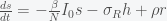

 , where
  and
and  . The trace of the matrix is
  so the sum of the eigenvalues is negative but the determinant is zero (since the rows sum to zero), and thus the product of the eigenvalues is zero. With a little calculation you can show that this system has two eigenvalues with negative real part and one zero eigenvalue. Thus, the fixed point is not linearly stable but could still be nonlinearly stable, which it probably is since the nonlinear terms are attracting.
 . Thus, as long as the reinfection rate is much smaller than the initial infection rate (which it seems to be), we are headed for a situation where Covid-19 is endemic and will just keep circulating around forever. It may have a seasonal variation like the flu, which is still not well understood and is beyond the simple SIRS equation. If we include death in the equations then there is no longer a nonzero fixed point and the dynamics will just leak slowly towards everyone dying. However, if the death rate is slow enough this will be balanced by births and deaths due to other causes.
 different possible hashes. What makes hashes useful are two properties. The first, as mentioned, is that it is a one-way function and the second is that two different inputs do not give the same hash, called collision avoidance. There have been decades of work on figuring out how to do this and institutions like the US National Institutes of Standards and Technology (NIST) actually publish hash standards like SHA-2.
  (i.e. fraction of planets with life) and this probability is uniform across the universe. Then if you search
  planets, the probability for the number of planets with life you will find is given by a Binomial distribution. The probability that there are
  , where
  is a factor (the binomial coefficient) such that the sum of
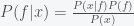
 . As expected, the posterior depends strongly on the prior. A convenient way to express the prior probability is to use a Beta distribution
 (*)
(*) is again a normalization constant (the Beta function). The mean of a beta distribution is given by
  and the variance, which is a measure of uncertainty, is given by
  . The posterior distribution for
 is a normalization factor. This is again a Beta distribution. The Beta distribution is called the conjugate prior for the Binomial because it’s form is preserved in the posterior.
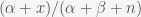 and
and  , respectively. Now let’s consider how our priors have updated. Suppose our prior was
  , which gives a uniform distribution for
  . The observation of a single planet has greatly reduced our uncertainty and we now expect about 1 in 5000 planets to have life. Now what happens if we find no planets. Then, our expected
  and
and  so our expected probability is zero with zero variance. The observation of a single planet increases our posterior to 1 in 10001 with about the same small variance. However, if we find a single planet out of much fewer observations like 100, then our expected probability for life would be even higher but with more uncertainty. In any case, Sara Seager’s intuition is correct – finding a planet would be a game breaker and not finding one shouldn’t really discourage us that much.
 it takes for an object traveling at constant velocity to reach its target is

 is the distance and
  is the velocity. This infinite series is technically called a geometric series because the ratio of two subsequent terms in the series is always the same. The terms are related geometrically like the volumes of n-dimensional cubes when you have halve the length of the sides (e.g. 1-cube (line and volume is length), 2-cube (square and volume is area), 3-cube (good old cube and volume), 4-cube ( hypercube and hypervolume), etc) .
 . So to compute the time it takes to travel the distance, we must compute:
 and obtain
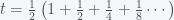


 . We then have the amazing fact that
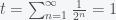
 that is less than 1. The more compact way to express this is
 , you get
  , which is infinity. Since
  for any
  you’ll get a negative number. Does this mean that the sum of an infinite number of positive numbers greater than 1 is a negative number? Well no because the series is only defined for
  , which is called the domain of convergence. If you go outside of the domain, you can still get an answer but it won’t be the answer to your question. You always need to be careful when you add and subtract infinite quantities. Depending on the circumstance it may or may not give you sensible answers. Getting that right is what math is all about.
 positive tests if the person is positive is
  , where
  is the cumulative distribution function of the Binomial distribution (i.e. probability that the number of Binomial distributed events is less than or equal to
  . We thus want to find the minimal
  and
and  . This means that we need to solve the constrained optimization problem: find the minimal
  ,
,  and
and  .
.  decreases and
  and treat them as some abstract quantity. In fact, I often just look at differential equations of the form
 is a solution, where
  is any constant number, because the derivative of an exponential function is an exponential function. One confusing aspect of discussing exponential growth with lay people is that the above equation is called a linear differential equation and often mathematicians or physicists will simply say the dynamics are linear or even the growth is linear, although what we really mean is that the describing equation is a linear differential equation, which has exponential growth or exponential decay if
  actually means is that every day
  , which is about 2.718. Now, while this is the most convenient number for mathematical manipulation, it is definitely not the most convenient number for intuition. A common alternative is to use 2 as the base of the exponent, rather than
  , which is only 10 million or so. But on day 31 you have 20 million and day 32 you have 40 million. It’s growing really fast.
 then
then  (i.e. the log of x in base 2 is 3). Log just gives you the power of an exponential (in that base). So the only difference between using base 2 versus base 10 is the rate of growth. For example
  , where
  . So an exponential process that is doubling every day is increasing by a factor of ten every 3.3 days.