Chat GPT and the end of human culture

I had a personal situation this past year that kept me from posting much but today I decided to sit down and write something – all by myself without any help from anyone or anything. I could have enlisted the help of Chat GPT or some other large language model (LLM) but I didn’t. These posts generally start out with a foggy idea, which then take on a life of their own. Part of my enjoyment of writing these things is that I really don’t know what they will say until I’m finished. But sometime in the near future I’m pretty sure that WordPress will have a little window where you can type an idea and a LLM will just write the post for you. At first I will resist using it but one day I might not feel well and I’ll try it and like it and eventually all my posts will be created by a generative AI. Soon afterwards, the AI will learn what I like to blog about and how often I do so and it will just start posting on it’s own without my input. Maybe most or all content will be generated by an AI.

These LLMs are created by training a neural network to predict the next word of a sentence, given the previous words, sentences, paragraphs, and essentially everything that has ever been written. The machine is fed some text and produces what it thinks should come next. It then compares its prediction with the actual answer and updates its settings (connection weights) based on some score of how well it did. When fed the entire corpus of human knowledge (or at least what is online), we have all seen how well it can do. As I have speculated previously (see here), this isn’t all too surprising given that the written word is relatively new in our evolutionary history. Thus, humans aren’t really all that good at it and there isn’t all that much variety in what we write. Once an AI has the ability to predict the next word, it doesn’t take much more tinkering to make it generate an entire text. The specific technology that made this generative leap is called a diffusion model, which I may describe in more technical detail in the future. But in the simplest terms, the model finds successive small modifications to transform the initial text (or image or anything) into pure noise. The model can then be run backwards starting from random noise to create text.

When all content is generated by AI, the AI will no longer have any human data on which to further train. Human written culture will then be frozen. The written word will just consist of rehashing of previous thoughts along with random insertions generated by a machine. If the AI starts to train on AI generated text then it could leave human culture entirely. Generally, when these statistical learning machines train on their own generated data they can go unstable and become completely unpredictable. Will the AI be considered conscious by then?

The probability of extraterrestrial life

Since, the discovery of exoplanets nearly 3 decades ago most astronomers, at least the public facing ones, seem to agree that it is just a matter of time before they find signs of life such as the presence of volatile gases in the atmosphere associated with life like methane or oxygen. I’m an agnostic on the existence of life outside of earth because we don’t have any clue as to how easy or hard it is for life to form. To me, it is equally possible that the visible universe is teeming with life or that we are alone. We simply do not know.

But what would happen if we find life on another planet. How would that change our expected probability for life in the universe? MIT astronomer Sara Seager once made an offhand remark in a podcast that finding another planet with life would make it very likely there were many more. But is this true? Does the existence of another planet with life mean a dramatic increase in the probability of life in the universe. We can find out by doing the calculation.

Suppose you believe that the probability of life on a planet is (i.e. fraction of planets with life) and this probability is uniform across the universe. Then if you search planets, the probability for the number of planets with life you will find is given by a Binomial distribution. The probability that there are planets is given by the expression , where is a factor (the binomial coefficient) such that the sum of from one to is 1. By Bayes Theorem, the posterior probability for (yes, that would be the probability of a probability) is given by

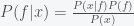
where . As expected, the posterior depends strongly on the prior. A convenient way to express the prior probability is to use a Beta distribution

(*)

where is again a normalization constant (the Beta function). The mean of a beta distribution is given by and the variance, which is a measure of uncertainty, is given by . The posterior distribution for after observing planets with life out of will be

where is a normalization factor. This is again a Beta distribution. The Beta distribution is called the conjugate prior for the Binomial because it’s form is preserved in the posterior.

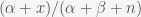Applying Bayes theorem in equation (*), we see that the mean and variance of the posterior become and , respectively. Now let’s consider how our priors have updated. Suppose our prior was , which gives a uniform distribution for on the range 0 to 1. It has a mean of 1/2 and a variance of 1/12. If we find one planet with life after checking 10,000 planets then our expected becomes 2/10002 with variance . The observation of a single planet has greatly reduced our uncertainty and we now expect about 1 in 5000 planets to have life. Now what happens if we find no planets. Then, our expected only drops to 1 in 10000 and the variance is about the same. So, the difference between finding a planet versus not finding a planet only halves our posterior if we had no prior bias. But suppose we are really skeptical and have a prior with and so our expected probability is zero with zero variance. The observation of a single planet increases our posterior to 1 in 10001 with about the same small variance. However, if we find a single planet out of much fewer observations like 100, then our expected probability for life would be even higher but with more uncertainty. In any case, Sara Seager’s intuition is correct – finding a planet would be a game breaker and not finding one shouldn’t really discourage us that much.

How to make a fast but bad COVID-19 test good

Among the myriad of problems we are having with the COVID-19 pandemic, faster testing is one we could actually improve. The standard test for the presence of SARS-CoV-2 virus uses PCR (polymerase chain reaction), which amplifies targeted viral RNA. It is accurate (high specificity) but requires relatively expensive equipment and reagents that are currently in short supply. There are reports of wait times of over a week, which renders a test useless for contact tracing.

An alternative to PCR is an antigen test that tests for the presence of protein fragments associated with COVID-19. These tests can in principle be very cheap and fast, and could even be administered on paper strips. They are generally much more unreliable than PCR and thus have not been widely adopted. However, as I show below by applying the test multiple times, the noise can be suppressed and a poor test can be made arbitrarily good.

The performance of binary tests are usually gauged by two quantities – sensitivity and specificity. Sensitivity is the probability that you test positive (i.e are infected) given that you actually are positive (true positive rate). Specificity is the probability that you test negative if you actually are negative (true negative rate). For a pandemic, sensitivity is more important than specificity because missing someone who is infected means you could put lots of people at risk while a false positive just means the person falsely testing positive is inconvenienced (provided they cooperatively self-isolate). Current PCR tests have very high specificity but relatively low sensitivity (as low as 0.7) and since we don’t have enough capability to retest, a lot of tested infected people could be escaping detection.

The way to make any test have arbitrarily high sensitivity and specificity is to apply it multiple times and take some sort of average. However, you want to do this with the fewest number of applications. Suppose we administer tests on the same subject, the probability of getting more than positive tests if the person is positive is , where is the cumulative distribution function of the Binomial distribution (i.e. probability that the number of Binomial distributed events is less than or equal to ). If the person is negative then the probability of  or fewer positives is . We thus want to find the minimal given a desired sensitivity and specificity, and . This means that we need to solve the constrained optimization problem: find the minimal under the constraint that , and 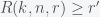. decreases and increases with increasing and vice versa for . We can easily solve this problem by sequentially increasing and scanning through until the two constraints are met. I’ve included the Julia code to do this below.  For example, starting with a test with sensitivity .7 and specificity 1 (like a PCR test), you can create a new test with greater than .95 sensitivity and specificity, by administering the test 3 times and looking for a single positive test. However, if the specificity drops to .7 then you would need to find more than 8 positives out of 17 applications to be 95% sure you have COVID-19.

 

using Distributions

function Q(k,n,q)
d = Binomial(n,q)
return 1 – cdf(d,k)
end

function R(k,n,r)
d = Binomial(n,1-r)
return cdf(d,k)
end

function optimizetest(q,r,qp=.95,rp=.95)

nout = 0
kout = 0

for n in 1:100
for k in 0:n-1
println(R(k,n,r),” “,Q(k,n,q))
if R(k,n,r) >= rp && Q(k,n,q) >= qp
kout=k
nout=n
break
end
end
if nout > 0
break
end
end

return nout, kout
end

Slides for Covid-19 talk

Here are my slides for my recent COVID-19 talk at the Centre for Applied Mathematics in BioScience and Medicine (CAMBAM). It’s an updated version of the one I gave to the FDA.

A Covid-19 Manhattan Project

Right now there are hundreds if not thousands of Covid-19 models floating out there. Some are better than others and some have much more influence than others and the ones that have the most influence are not necessarily the best. There must be a better way of doing this. The world’s greatest minds convened in Los Alamos in WWII and built two atomic bombs. Metaphors get thrown around with reckless abandon but if there ever was a time for a Manhattan project, we need one now. Currently, the world’s scientific community has mobilized to come up with models to predict the spread and effectiveness of mitigation efforts, to produce new therapeutics and to develop new vaccines. But this is mostly going on independently.

Would it be better if we were to coordinate all of this activity. Right now at the NIH, there is an intense effort to compile all the research that is being done in the NIH Intramural Program and to develop a system where people can share reagents and materials. There are other coordination efforts going on worldwide as well.  This website contains a list of open source computational resources.  This link gives a list of data scientists who have banded together. But I think we need a world wide plan if we are ever to return to normal activity. Even if some nation has eliminated the virus completely within its borders there is always a chance of reinfection from outside.

In terms of models, they seem to have very weak predictive ability. This is probably because they are all over fit. We don’t really understand all the mechanisms of SARS-CoV-2 propagation. The case or death curves are pretty simple and as Von Neumann or Ulam or someone once said, “give me 4 parameters and I can fit an elephant, give me 5 and I can make it’s tail wiggle.” Almost any model can fit the curve but to make a projection into the future, you need to get the dynamics correct and this I claim, we have not done. What I am thinking of proposing is to have the equivalent of FDA approval for predictive models. However, instead of a binary decision of approval non-approval, people could submit there models for a predictive score based on some cross validation scheme or prediction on a held out set. You could also submit as many times as you wish to have your score updated. We could then pool all the models and produce a global Bayesian model averaged prediction and see if that does better. Let me know if you wish to participate or ideas on how to do this better.

Covid-19 talk

Here are the slides for my webinar at FDA today .

COVID-19 Paper

First draft of our paper can be downloaded from this link.  I’ll post more details about it later.

Global prediction of unreported SARS-CoV2 infection from observed COVID-19 cases

Carson C. Chow 1*, Joshua C. Chang 2,3, Richard C. Gerkin 4*, Shashaank Vattikuti 1*

1Mathematical Biology Section, LBM, NIDDK, National Institutes of Health2Epidemiology and Biostatistics Section, Rehabilitation Medicine, Clinical Center, National Institutes of Health 3 mederrata 4 School of Life Sciences, Arizona State University

*For correspondence contact carsonc@nih.gov, josh@mederrata.com, rgerkin@asu.edu, vattikutis@nih.gov

Summary: Estimation of infectiousness and fatality of the SARS-CoV-2 virus in the COVID-19 global pandemic is complicated by ascertainment bias resulting from incomplete and non-representative samples of infected individuals.  We developed a strategy for overcoming this bias to obtain more plausible estimates of the true values of key epidemiological variables.  We fit mechanistic Bayesian latent-variable SIR models to confirmed COVID-19 cases, deaths, and recoveries, for all regions (countries and US states) independently. Bayesian averaging over models, we find that the raw infection incidence rate underestimates the true rate by a factor, the case ascertainment ratio CARt that depends upon region and time. At the regional onset of COVID-19, the predicted global median was 13 infections unreported for each case confirmed (CARt = 0.07 C.I. (0.02, 0.4)). As the infection spread, the median CARt rose to 9 unreported cases for every one diagnosed as of April 15, 2020 (CARt = 0.1 C.I. (0.02, 0.5)).  We also estimate that the median global initial reproduction number R0 is 3.3 (C.I (1.5, 8.3)) and the total infection fatality rate near the onset is 0.17% (C.I. (0.05%, 0.9%)). However the time-dependent reproduction number Rt and infection fatality rate as of April 15 were 1.2 (C.I. (0.6, 2.5)) and 0.8% (C.I. (0.2%,4%)), respectively.  We find that there is great variability between country- and state-level values.  Our estimates are consistent with recent serological estimates of cumulative infections for the state of New York, but inconsistent with claims that very large fractions of the population have already been infected in most other regions.  For most regions, our estimates imply a great deal of uncertainty about the current state and trajectory of the epidemic.

 

Covid-19 modeling

I have officially thrown my hat into the ring and joined the throngs of would-be Covid-19 modelers to try to estimate (I deliberately do not use predict) the progression of the pandemic. I will pull rank and declare that I kind of do this type of thing for a living. What I (and my colleagues whom I have conscripted) are trying to do is to estimate the fraction of the population that has the SARS-CoV-2 virus but has not been identified as such. This was the goal of the Lourenco et al. paper I wrote about previously that pulled me into this pit of despair. I argued that fitting to deaths alone, which is what they do, is insufficient for constraining the model and thus it has no predictive ability. What I’m doing now is seeing whether it is possible to do the job if you fit not only deaths but also the number of cases reported and cases recovered. You then have a latent variable model where the observed variables are cases, cases that die, and cases that recover, and the latent variables are the infected that are not identified and the susceptible population. Our plan is to test a wide range of models with various degrees of detail and complexity and use Bayesian Model Comparison to see which does a better job. We will apply the analysis to global data. We’re getting numbers now but I’m not sure I trust them yet so I’ll keep computing for a few more days. The full goal is to quantify the uncertainty in a principled way.

2020-04-06: edited for purging typos

Response to Oxford paper on covid-19

Here is my response to the paper from Oxford (Lourenco et al.) arguing that novel coronavirus infection may already be widespread in the UK and Italy.  The result is based on fitting a disease spreading model, called an SIR model, to the cumulative number of deaths. SIR models usually consist of ordinary differential equations (ODEs) for the fraction of people in a given population who are susceptible to the infectious agent (S), the number infected (I),  and the number recovered (R). There is one other state in the model, which is the fraction who die from the disease (D).  The SIR model considers transitions between these states.  In the case of ODEs, the states are treated as continuous quantities, which is not a bad approximation for a large population, and each equation in the model describes the rate of change of a state (hence differential equation).  There are parameters in the model governing the rate of different interactions in each  equation, for example there is a parameter for the rate of increase in S whenever an S interacts with an I, and then there is a rate of loss of an I, which transitions into either R or D.  The Oxford group model D somewhat differently.  Instead of a transition from I into D they consider that a fraction of (1-S) will die with some delay between time of infection and death.

They estimate the model parameters by fitting the model to the cumulative number of deaths.  They did this instead of fitting directly to I because that is unreliable as many people who have Covid-19 have not been tested. They also only fit to the first 15 days from the first recorded death since they want to model what happens before social distancing was implemented.  They find that the model is consistent with a scenario where the probability that an infected person gets severe enough to be flagged is low and thus the disease is much more wide spread than expected. I redid the analysis without assuming that the parameters need to have particular values (called priors in Bayesian inference and machine learning) and showed that a wide range of parameters will fit the data. This is because the model is under-constrained by death data alone so even unrealistic parameters can work.  To be fair, the authors only proposed that this is a possibility and thus the population should be tested for anti-bodies to the coronavirus (SARS-CoV-2) to see if indeed there may already be herd immunity in place. However, the press has run with the result and that is why I think it is important to examine the result more closely.

The tragedy of low probability events

We live in an age of fear and yet life (in the US at least) is the safest it has ever been. Megan McArdle blames coddling parents and the media in a Washington Post column. She argues that cars and swimming pools are much more dangerous than school shootings and kidnappings yet we mostly ignore the former and obsess about the latter. However, to me dying from an improbable event is just so much more tragic than dying from an expected one. I would be much less despondent meeting St. Peter at the Pearly Gates if I happened to expire from cancer or heart disease than if I were to be hit by an asteroid while weeding my garden. We are so scared now because we have never been safer. We would fear terrorist attacks less if they were more frequent. This is the reason that I would never want a major increase in lifespan. I most certainly would like to last long enough to see my children become independent but anything beyond that is bonus time. Nothing could be worse to me than immortality. The pain of any tragedy would be unbearable. Life would consist of an endless accumulation of sad memories. The way out is to forget but that to me is no different from death. What would be the point of living forever if you were to erase much of it. What would a life be if you forgot the people and things that you loved? To me that is no life at all.

Optimizing luck

Each week on the NPR podcast How I Built This, host Guy Raz interviews a founder of a successful enterprise like James Dyson or Ben and Jerry. At the end of most segments, he’ll ask the founder how much of their success do they attribute to luck and how much to talent. In most cases, the founder will modestly say that luck played a major role but some will add that they did take advantage of the luck when it came. One common thread for these successful people is that they are extremely resilient and aren’t afraid to try something new when things don’t work at first.

There are two ways to look at this. On the one hand there is certainly some selection bias. For each one of these success stories there are probably hundreds of others who were equally persistent and worked equally hard but did not achieve the same success. It is like the infamous con where you send 1024 people a two outcome prediction about a stock.  The prediction will be correct in 512 of them so the next week you send those people another prediction and so on. After 10 weeks, one person will have received the correct prediction 10 times in a row and will think you are infallible. You then charge them a King’s ransom for the next one.

Yet, it may be possible to optimize luck and you can see this with Jensen’s inequality. Suppose represents some combination of your strategy and effort level and is your outcome function.  Jensen’s inequality states that the average or expectation value of a convex function (e.g. a function that bends upwards) is greater than (or equal to) the function of the expectation value. Thus, . In other words, if your outcome function is convex then your average outcome will be larger just by acting in a random fashion. During “convex” times, the people who just keep trying different things will invariably be more successful than those who do nothing. They were lucky (or they recognized) that their outcome was convex but their persistence and willingness to try anything was instrumental in their success. The flip side is that if they were in a nonconvex era, their random actions would have led to a much worse outcome. So, do you feel lucky?

Technology and inference

In my previous post, I gave an example of how fake news could lead to a scenario of no update of posterior probabilities. However, this situation could occur just from the knowledge of technology. When I was a child, fantasy and science fiction movies always had a campy feel because the special effects were unrealistic looking. When Godzilla came out of Tokyo Harbour it looked like little models in a bathtub. The Creature from the Black Lagoon looked like a man in a rubber suit. I think the first science fiction movie that looked astonishing real was Stanley Kubrick’s 1968 masterpiece 2001: A Space Odyssey, which adhered to physics like no others before and only a handful since. The simulation of weightlessness in space was marvelous and to me the ultimate attention to detail was the scene in the rotating space station where a mild curvature in the floor could be perceived. The next groundbreaking moment was the 1993 film Jurassic Park, which truly brought dinosaurs to life. The first scene of a giant sauropod eating from a tree top was astonishing. The distinction between fantasy and reality was forever gone.

The effect of this essentially perfect rendering of anything into a realistic image is that we now have a plausible reason to reject any evidence. Photographic evidence can be completely discounted because the technology exists to create completely fabricated versions. This is equally true of audio tapes and anything your read on the Internet. In Bayesian terms, we now have an internal model or likelihood function that any data could be false. The more cynical you are the closer this constant is to one. Once the likelihood becomes insensitive to data then we are in the same situation as before. Technology alone, in the absence of fake news, could lead to a world where no one ever changes their mind. The irony could be that this will force people to evaluate truth the way they did before such technology existed, which is that you believe people (or machines) that you trust through building relationships over long periods of time.

Fake news and beliefs

Much has been written of the role of fake news in the US presidential election. While we will never know how much it actually contributed to the outcome, as I will show below, it could certainly affect people’s beliefs. Psychology experiments have found that humans often follow Bayesian inference – the probability we assign to an event or action is updated according to Bayes rule. For example, suppose is the probability we assign to whether climate change is real; 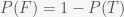is our probability that climate change is false. In the Bayesian interpretation of probability, this would represent our level of belief in climate change. Given new data (e.g. news), we will update our beliefs according to

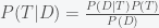
What this means is that our posterior probability or belief that climate change is true given the new data, , is equal to the probability that the new data came from our internal model of a world with climate change (i.e. our likelihood), multiplied by our prior probability that climate change is real, divided by the probability of obtaining such data in all possible worlds, . According to the rules of probability, the latter is given by , which is the sum of the probability the data came from a world with climate change and that from one without.

This update rule can reveal what will happen in the presence of new data including fake news. The first thing to notice is that if is zero, then there is no update. In this binary case, this means that if we believe that climate change is absolutely false or true then no data will change our mind. In the case of multiple outcomes, any outcome with zero prior (has no support) will never change. So if we have very specific priors, fake news is not having an impact because no news is having an impact. If we have nonzero priors for both true and false then if the data is more likely from our true model then our posterior for true will increase and vice versa. Our posteriors will tend towards the direction of the data and thus fake news could have a real impact.

For example, suppose we have an internal model where we expect the mean annual temperature to be 10 degrees Celsius with a standard deviation of 3 degrees if there is no climate change and a mean of 13 degrees with climate change. Thus if the reported data is mostly centered around 13 degrees then our belief of climate change will increase and if it is mostly centered around 10 degrees then it will decrease. However, if we get data that is spread uniformly over a wide range then both models could be equally likely and we would get no update. Mathematically, this is expressed as – if  then . From the Bayesian update rule, the posterior will be identical to the prior. In a world of lots of misleading data, there is no update. Thus, obfuscation and sowing confusion is a very good strategy for preventing updates of priors. You don’t need to refute data, just provide fake examples and bury the data in a sea of noise.

 

Probability of gun death

The tragedy in Oregon has reignited the gun debate. Gun control advocates argue that fewer guns mean fewer deaths while gun supporters argue that if citizens were armed then shooters could be stopped through vigilante action. These arguments can be quantified in a simple model of the probability of gun death, :

where is the probability of having a gun,  is the probability of being a criminal or  mentally unstable enough to become a shooter,  is the probability of effective vigilante action, and is the probability of accidental death or suicide.  The probability of being killed by a gun is given by the probability of someone having a gun times the probability that they are unstable enough to use it. This is reduced by the probability of a potential victim having a gun times the probability of acting effectively to stop the shooter. Finally, there is also a probability of dying through an accident.

The first derivative of with respect to is and the second derivative is negative. Thus, the minimum of cannot be in the interior  and must be at the boundary. Given that when and when , the absolute minimum is found when no one has a gun. Even if vigilante action was 100% effective, there would still be gun deaths due to accidents. Now, some would argue that zero guns is not possible so we can examine if it is better to have fewer guns or more guns.  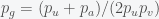is maximal at . Thus, unless is greater than one half then even in the absence of accidents there is no situation where increasing the number of guns makes us safer. The bottom line is that if we want to reduce gun deaths we should either reduce the number of guns or make sure everyone is armed and has military training.

 

 

 

Sampling from a probability distribution

When simulating any system with randomness, sampling from a probability distribution is necessary. Usually, you’ll just need to sample from a normal or uniform distribution and thus can use a built-in random number generator. However, for the time when a built-in function does not exist for your distribution, here’s a simple algorithm.

Let’s say you have some probability density function (PDF) on some domain and you want to generate a set of numbers that follows this probability law. This is actually very simple to do although those new to the field may not know how. Generally, any programming language or environment has a built-in random number generator for real numbers (up to machine precision) between 0 and 1. Thus, what you want to do is to find a way to transform these random numbers, which are uniformly distributed on the domain to the random numbers you want. The first thing to notice is that the cumulative distribution function (CDF) for your PDF, is a function that ranges over the interval , since it is a probability. Thus, the algorithm is: 1) generate a random number between o and 1, and 2) plug it into the inverse of . The numbers you get out satisfy your distribution (i.e. ).

If you’re lucky enough to have a closed form expression of the inverse of the CDF then you can just plug the random numbers directly into your function, otherwise you have to do a little more work. If you don’t have a closed form expression for the CDF then you can just solve the equation for . Newton’s method will generally converge very quickly.  You just loop over the command x = x – (P(x)-r)/rho(x) until you reach the tolerance you want. If you don’t have a closed form expression of the CDF then the simplest way is construct the CDF numerically by computing the N dimensional vector , for some discretization parameter such that  .  If the PDF is defined on the entire real line then you’ll have to decide on what you want the minimum and maximum (through ) to be. If the distribution has thin tails, then you just need to go out until the probability is smaller than your desired error tolerance. You then find the index such that is closest to (i.e. in Julia you could use findmin(abs(v[j]-r))) and your random number is .

Here is why the algorithm works. What we are doing is transforming the PDF of , which we can call , to the desired PDF for . The transformation we use is . Thus, or . Now, is just 1 on the interval and is the PDF of as expected. Thus, inverting the CDF for uniform random numbers always gives you a new set of random numbers that satisfies the new PDF. Trivial perhaps, but really useful.

Erratum: 2019-04-05.  It was pointed out to me that my algorithm involving direct summation of the CDF had some errors.  I hope they have now been corrected.

New paper on path integrals

Carson C. Chow and Michael A. Buice. Path Integral Methods for Stochastic Differential Equations. The Journal of Mathematical Neuroscience,  5:8 2015.

Abstract: Stochastic differential equations (SDEs) have multiple applications in mathematical neuroscience and are notoriously difficult. Here, we give a self-contained pedagogical review of perturbative field theoretic and path integral methods to calculate moments of the probability density function of SDEs. The methods can be extended to high dimensional systems such as networks of coupled neurons and even deterministic systems with quenched disorder.

This paper is a modified version of our arXiv paper of the same title.  We added an example of the stochastically forced FitzHugh-Nagumo equation and fixed the typos.

Code platform update

It’s a week away from 2015, and I have transitioned completely away from Matlab. Julia is winning the platform attention battle. It is very easy to code in and it is very fast. I just haven’t gotten around to learning python much less pyDSTool (sorry Rob). I kind of find the syntax of Python (with all the periods between words) annoying. Wally Xie and I have also been trying to implement some of our MCMC runs in Stan but we have had trouble making it work.  Our model requires integrating ODEs and the ODE solutions from Stan (using our own solver) do not match our Julia code or the gold standard XPP. Maybe we are missing something obvious in the Stan syntax but our code is really very simple. Thus, we are going back to doing our Bayesian posterior estimates in Julia. However, I do plan to revisit Stan if they (or we) can write a debugger for it.

MCMC for linear models

I’ve been asked in a comment to give a sample of pseudo code for an MCMC algorithm to fit a linear model to some data. See here for the original post on MCMC. With a linear model, you can write down the answer in closed form (see here), so it is a good model to test your algorithm and code.  Here it is in pseudo-Julia code:

#  initial guess for parameters a and b 
a=0
b=0

# construct chi squared, where D is the data vector and x is the vector of the 
# independent quantity

chi = norm(D - (a*x +b))^2;

for n = 1 : total;
# Make random guesses for new normally distributed a and b with mean old a and b 
# and standard deviation asig and bsig

at = a + asig * randn()
bt = b + bsig * randn()

chit = norm(D - (at*x + bt))^2;

# Take ratio of likelihoods, sigma is the data uncertainty
ratio=exp((-chit + chi)/(2*sigma^2));

# Compare the ratio to a uniform random number between 0 and 1, 
# keep new parameters if ratio exceeds random number
if rand() < ratio
a = at;
b = bt;
chi = chit;
end

end

# Keep running until convergence

Big Data backlash

I predicted that there would be an eventual push back on Big Data and it seems that it has begun. Gary Marcus and Ernest Davis of NYU had an op-ed in the Times yesterday outlining nine issues with Big Data. I think one way to encapsulate many of the critiques is that you will never be able to do true prior free data modeling. The number of combinations in a data set grows as the factorial of the number of elements, which grows faster than an exponential. Hence, Moore’s law can never catch up. At some point, someone will need to exercise some judgement in which case Big Data is not really different from the ordinary data that we deal with all the time.

The myth of the single explanation

I think one of the things that tends to lead us astray when we try to understand complex phenomena like evolution, disease, or the economy, is that we have this idea that they must have a single explanation. For example, recently two papers have been published in high profile journals trying to explain mammal monogamy. Although monogamy is quite common in birds it only occurs in 5% of mammals. Here is Carl Zimmer’s summary.  The study in Science, which surveyed 2545 mammal species, argued that monogamy arises when females are solitary and sparse. Males must then commit to one since dates are so hard to find. The study in PNAS examined 230 primate species, for which monogamy occurs at the higher rate of 27%, and used Bayesian inference to argue that monogamy arises to prevent male infanticide. It’s better to help out at home rather than go around killing other men’s babies. Although both of these arguments are plausible, there need not be a single universal explanation. Each species could have its own set of circumstances that led to monogamy involving these two explanations and others. However, while we should not be biased towards a single explanation, we shouldn’t also throw up our hands like Hayek and argue that no complex phenomenon can be understood. Some phenomena will have simpler explanations than others but since the Kolmogorov complexity is undecidable there is no algorithm that can tell you which is which. We will just have to struggle with each problem as it comes.