My 8th grade daughter had her final (distance learning) science quiz this week on work, or as it is called in her class, the scientific definition of work. I usually have no idea what she does in her science class since she rarely talks to me about school but she so happened to mention this one tidbit because she was proud that she didn’t get fooled by what she thought was a trick question. I’ve always believed that work, as in force times displacement (not the one where you produce economic value), is one of the most useless concepts in physics and should not be taught to anyone until they reach graduate school, if then. It is a concept that has long outlived its usefulness and all it does now is to convince students that science is just a bunch of concepts invented to confuse you. The problem with science education in general is that it is taught as a set of facts and definitions when the only thing that kids need to learn is that science is about trying to show something is true using empirical evidence. My daughter’s experience is evidence that science education in the US has room for improvement.
Work, as defined in science class, is just another form of energy, and the only physics that should be taught to middle school kids is that there are these quantities in the universe called energy and momentum and they are conserved. Work is just the change in energy of a system due to a force moving something. For example, the work required to lift a mass against gravity is the distance the mass was lifted multiplied by the force used to move it. This is where it starts to get a little confusing because there are actually two reasons you need force to move something. The first is because of Newton’s First Law of inertia – things at rest like to stay at rest and things in motion like to stay in motion. In order to move something from rest you need to accelerate it, which requires a force and from Newton’s second law, Force equals mass times acceleration, or F = ma. However, if you move something upwards against the force of gravity then even to move at a constant velocity you need to use a force that is equal to the gravitational force pulling the thing downwards, which from Newton’s law of gravitation is given by 


In the first part of my daughter’s quiz, she was asked to calculate the energy consumed by several appliances in her house for one week. She had to look up how much power was consumed by the refrigerator, computer, television and so forth on the internet. Power is energy per unit time so she computed the amount of energy used by multiplying the power used by the total time the device is on per week. In the second part of the quiz she was asked to calculate how far she must move to power those devices. This is actually a question about conservation of energy and to answer the question she had to equate the energy used with the work definition of force times distance traveled. The question told her to use gravitational force, which implies she had to be moving upwards against the force of gravity, or accelerating at g if moving horizontally, although this was not specifically mentioned. So, my daughter took the energy used to power all her appliances and divided it by the force, i.e. her mass times g, and got a distance. The next question was, and I don’t recall exactly how it was phrased but something to the effect of: “Did you do scientifically defined work when you moved?”
Now, in her class, she probably spent a lot of time examining situations to distinguish work from non-work. Lifting a weight is work, a cat riding a Roomba is not work. She learned that you did no work when you walked because the force was perpendicular to your direction of motion. I find these types of gotcha exercises to be useless at best and in my daughter’s case completely detrimental. If you were to walk by gliding along completely horizontally with absolutely no vertical motion at a constant speed then yes you are technically not doing mechanical work. But your muscles are contracting and expanding and you are consuming energy. It’s not your weight times the distance you moved but some very complicated combination of metabolic rate, muscle biochemistry, energy losses in your shoes, etc. Instead of looking at examples and identifying which are work and which are not, it would be so much more informative if they were asked to deduce how much energy would be consumed in doing these things. The cat on the Roomba is not doing work but the Roomba is using energy to turn an electric motor that has to turn the wheel to move the cat. It has to accelerate from standing still and also gets warm, which means some of the energy is wasted to heat. A microwave oven uses energy because it must generate radio waves. Boiling water takes energy because you need to impart random kinetic energy to the water molecules. A computer uses energy because it needs to send electrons through transistors. Refrigerators work by using work energy to pump the heat energy from the inside to the outside. You can’t cool a room by leaving the refrigerator door open because you will just pump heat around in a circle and some of the energy will be wasted as extra heat.
My daughter’s answer to the question of was work done was that no work was done because she interpreted movement to be walking horizontally and she knew from all the gotcha examples that walking was not work. She read to me her very legalistically parsed paragraph explaining her reasoning, which made me think that while science may not be in her future, law might be. I tried to convince her that in order for the appliances to run, energy had to come from somewhere so she must have done some work at some point in her travels but she would have no part of it. She said it must be a trick question so the answer has to not make sense. She proudly submitted the quiz convinced more then ever that her so-called scientist Dad is a complete and utter idiot.
 , with a PCR test with 100% sensitivity, which means we do not miss anyone who is positive but we could have false positives. The number of positives we will find is
  , where
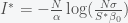
  is the prevalence of infectious individuals in a given population. If positive individuals are isolated from the rest of the population until they are no longer infectious with probability
  , then the rate of reduction in prevalence is
  . To reduce the pandemic, this number needs to be higher than the rate of pandemic growth, which is given by
  , where
  is the fraction of the population susceptible to SARS-CoV-2 infection and
  is the rate of transmission from an infected individual to a susceptible upon contact. Thus, to reduce the pandemic, we need to test at a rate higher than
  .
. , where
  is the mean reproduction number, which is probably around 3.7 and
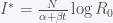
  is the mean rate of becoming noninfectious, which is probably around 10 to 20 days. This gives an estimate of
  to be somewhere around 0.3 per day. Thus, in the early stages of the pandemic, we would need to test everyone at least two or three times per week, provided positives are isolated. However, if people wear masks and avoid crowds then
 (SIR model)
 is the total number of people in the population of interest. Here,
  and
and  are in units of number of people. The left hand sides of these equations are derivatives with respect to time, or rates. They have dimensions or units of people per unit time, say day. From this we can infer that
  . If there was one infected person in a population of a hundred, then if you were to interact completely randomly with everyone then the chance you would run into an infected person is 1/100. Actually, it would be 1/99 but in a large population, the one becomes insignificant and you can round up. Right away, we can see a problem with this assumption. I interact regularly with perhaps a few hundred people per week or month but the chance of me meeting a person that had just come from Australia in a typical week is extremely low. Thus, it is not at all clear what we should use for
  . The rate of change of
  . These terms all have units of person per day. Once you understand the basic principles of constructing differential equations, you can model anything, which is what I like to do. For example, I modeled the temperature dynamics of my house this winter and used it to optimize my thermostat settings. In a post from a long time ago, I used it to model how best to boil water.
 is some nice function like
  or
or  . However, you can solve them numerically on a computer or infer properties of the dynamics directly without actually solving them. For example, if
  is initially greater than
  is always negative (rate of change is negative), it will decrease in time. As
  . This is a stationary point of
 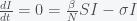 (Stationary condition)
 or
or  . The
. The  point is not a peak but just reflects the fact that there is no epidemic if there are no infections. The other condition gives the peak:
 then the pandemic will begin to decline. This is usually expressed as the fraction of those infected and no longer susceptible,
  . The 70% number you have heard is because
  is approximately 70% for
  , the presumed value for Covid-19.
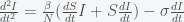
 at the peak, the curvature is
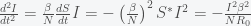
 is small compared to
  . However, this would also mean we are already at the herd immunity threshold, which our paper and recent anti-body surveys predict to be unlikely given what we know about
  ,where
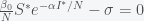
 , then
 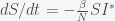 , which has solution
 (S)
(S)
 is given by equation (S). Substituting this into the (Stationary Condition) above then gives
  or
or
 is creeping upwards back to it’s original value.
 days! In other words, the pandemic will keep circling the world forever since over that time span, babies will be born and grow up. Most likely, it will become less virulent and will just join the panoply of diseases we currently live with like the various varieties of the common cold (which are also corona viruses) and the flu.