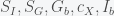
This is the third post on Bayesian inference. The other two are here and here. This probably should be the first one to read if you are completely unfamiliar with the topic. Suppose you are trying to model some system and you have a model that you want to match some data. The model could be a function, a set of differential equations, or anything with parameters that can be adjusted. To make this concrete, consider this classic differential equation model of the response of glucose to insulin in the blood:

![\dot X = c_X[I(t) - X -I_b]](https://s0.wp.com/latex.php?latex=%5Cdot+X+%3D+c_X%5BI%28t%29+-+X+-I_b%5D&bg=f5f6f7&fg=444444&s=0&c=20201002)
where 


The first question to answer is what do you mean by fitting the model at those time points. This is by no means simple to answer and the results will change depending on how you answer it. The standard procedure is to assign some error if the model does not go through the points and try to minimize the error. The most common error function is the mean square error, which we can write as
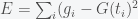
where 


Now, if you also want some sort of estimate of how good your fit is and what sort of uncertainty is associated with your estimate then you’ll need to use statistics. The starting point is to assume some probability distribution for your errors. Generally, a normal distribution is sufficient and you can always check if it was a good assumption after the fact by looking at the error distribution after you fit the data. In some cases, a simple transformation like taking the log will render the errors to be normal. So, suppose the error obeys a normal with zero mean and standard deviation 

Now, the model points 

where 
This is where the great divide between Bayesian and frequentist statistics comes in. The frequentists, led by Ronald Fisher, believe that probabilities can only be assigned to random variables, like the error, and that parameters of the model are fixed. So in their view, there is some optimal set of parameters out there that is obscured by random noise. So parameters cannot have errors attached to them. What you say instead is that given some set of parameters, this is the range of data values you would expect. You then try to find the parameters such that the expected data values bracket the measured data. It’s kind of a backwards way of thinking and is why statistics is so hard to understand, especially if you come from a dynamical systems/applied math background.
The Bayesian point of view, championed by Harold Jeffreys and Edwin Jaynes, is that everything can be assigned a probability. It simply represents some level of uncertainty you have about something. So parameters have probability distributions. The Bayesian approach is to “normalize” the likelihood function and turn it into a probability. This is done using Bayes’s rule
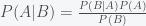
so now the probability of the parameters given the data points 
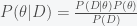
where 


One of the reasons it took the Bayesian approach so long to be accepted is that it was very difficult to compute the posterior. The evidence can be written as

which is an integral of the likelihood over the prior distribution of the parameters. In other words, to compute the posterior distribution you have to run the model over the entire parameter space you are interested in and sum that all up. This takes a lot of computational power but now any desktop machine can easily handle it. In fact, the easiest way to compute the posterior is to use the Markov Chain Monte Carlo method which I posted on earlier. What you do is simply keep all the parameter sets generated during a run (after some burn in period). The stationary distribution of the MCMC is the posterior probability distribution. In other words, instead of just keeping the parameter sets that minimized the error, you just save all the parameters generated by the MCMC run. The histogram of them is the posterior density. You can then take the mode, median or mean of the posterior as your best estimate. To get the error you can take the standard deviation of the posterior or the interval between 10 and 90 percent and so forth.
One of the biggest open questions in this approach is that there are no good theorems about the convergence rate of the MCMC. So, you really have no idea how long you have to run. This again is where fast computers partially saves you. I simply run for a long time and wait until nothing much changes and go with that. It’s no worse than using any optimization algorithm when you don’t know if you’ve reached a minimum. The last thing I will say is that you can use a method called parallel tempering, which is like simulated annealing, to speed up the posterior computation and also do model comparison in the same run. I’ll give the details of parallel tempering in the next post.

Actually, to my surprise, they are covering Bayesian statistics in medical school AGAIN, this time with an emphasis on pre-test vs. post-test probability and that the prevalence of the disease in the population really matters (not just the specificity of the test). They always sort of gloss over Bayes Theorem itself but they do a reasonably good job of getting the essential ideas across, especially as applied to interpreting and applying literature information to the patients.
Score one for Bayesians in medical school – except that the med students complain like crazy anytime “useless” things like Bayes’ Theorem are presented…)
LikeLike
great article!
i am approaching from only few weeks to machine learning and i’m lookiing for simple, clean and well-written articles, write more about bayesian inference!
LikeLike
Thanks, I have written some other posts, which you can find under the topic Bayes.
LikeLike
Love your posts on Bayesian inference as well! Great stuff and keep it up! Super helpful and well written!
LikeLike
This was very helpful …..I am an undergraduate student and need help to implement this in matlab.
Is it possible to implement this in Mat lab? Please post more information if any about the same model in Matlab.
Thankyou.
LikeLike
The post on Markov Chain Monte Carlo method has pseudo matlab code.
LikeLike
There’s one thing I still find confusing. You state that ‘a’ in your MCMC algorithm is the standard deviation of the parameter value, which is the standard deviation of the posterior probability density for the parameter. But to determine the posterior probability density you need to run the MCMC which in itself contains information about the posterior.
LikeLike
Oh, and is the Metropolis algorithm the same as the Metropolis-Hastings algorithm?
LikeLike
The stationary distribution of the MCMC is the posterior distribution. In some sense it turns the guess distribution into the posterior. It is not circular if that is what you are worried about. You can stick any guess distribution in and the same posterior will arise once you have reached convergence.
The Metropolis algorithm assumes that the guess distribution is symmetric (i.e. prob of guess given current state is the same as prob of current state given the guess). If this distribution is not symmetric then you use the Metropolis-Hastings algorithm. You can find the formula in any text book or Wikipedia.
LikeLike
[…] data analysis project where I need to manipulate very large matrices. It is true that we can now do Bayesian inference and model comparison on larger models. However, the curse of dimensionality strongly works […]
LikeLike
[…] to get a posterior probability). For a more technical treatment of Bayesian inference, see here. I posted previously (see here) that I thought that drastic differences in prior probabilities […]
LikeLike
Wonderful posts. Many things are getting clearer on Posterior Probability. I would you to relate it to Machine learning.
LikeLike