This is the follow up post to my earlier one on the Markov Chain Monte Carlo (MCMC) method for fitting models to data. I really should have covered Bayesian parameter estimation before this post but as an inadvertent demonstration of the simplicity of the Bayesian approach I’ll present these ideas in random order. Although it won’t be immediately apparent in this post, the MCMC is the only computational method you ever really need to learn to do all Bayesian inference.
It often comes up in biology and other fields that you have several possible models that could explain some data and you want to know which model is best. The first thing you could do is to see which model fits the data best. However, if a model has more parameters then certainly it will fit the model better. You could always have a model with as many parameters as data points and that would fit the data perfectly. So, it is necessary to balance how good you fit the data with the complexity of the model. There have been several proposals to address this issue. For example, the Akaike Information Criterion (AIC) or Bayes Information Criterion (BIC). However, as I will show here, these criteria are just approximations to Bayesian model comparison.
So suppose you have a set of data, which I will denote by D. This could be any set of measurements over any domain. For example it could be a time series of points such as the amount of glucose in the blood stream after a meal measured at each minute. We then have some proposed models that could fit the data and we want to know which is the best model. The model could be a polynomial, a differential equation or anything. Let’s say we have two models M1 and M2. The premise behind Bayesian inference is that anything can be assigned a probability so what we want to assess is the probability of a model given the data D. The model with the highest probability is then the most likely model. So we want to evaluate P(M1 |D) and compare it to P(M2|D). A frequentist could not do this because only random variables can be assigned probabilities and in fact there is no systematic way to evaluate models using frequentist statistics.
Now, how do you valuate P(M|D)? This is where Bayes rule comes in

where P(D|M) is the likelihood function, P(M) is the prior probability for the model and P(D) is the evidence.
This is also generally where people’s eyes start to glaze over. They can’t really see why simply rewriting probability can be of any use. The whole point is that while it is not clear how to estimate the probability of a model given the data, it is just a matter of computation to obtain the probability that the data would arise given a model i.e. P(D|M). However, there is one problem with equation (*) and that is it is not clear how to compute P(D), which is the probability of data marginalized over all models! The finesse around this problem is to look at odds ratios. So the odds ratio of M1 compared to M2 is given by
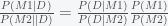
The ratio 

The next move is what fuels a massive debate between Bayesians and frequentists. Suppose each model depends on a set of parameters denoted by 

So what does this mean? Well it says that the probability that the data came from a model, is the “average” performance of a model “weighted” by the prior probability of the parameters. So, now you can see why this step is so controversial. It suggests that a model is only as good as the prior probability for the parameters of the model. The Bayesian viewpoint is that even if some model has a set of parameters that makes the model fit exactly to the data, if you have no idea where those parameters are then that model is not very good.
But there is even more to this. How good a model is also depends on how “broad” the prior distribution is compared to the likelihood function because the “overlap” between the two functions in the integrand of the integral in (**) determines how large the probability is. As a simple way to see this suppose there is one parameter and the prior for the parameter has the form
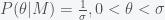
Then the likelihood for the model is given by

Now suppose that the likelihood is a single peaked function with a maximum likelihood value of L. Then we can rewrite the model likelihood as 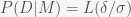


If we take the log of the likelihood we get

which can be compared to the BIC and AIC. So to compare two models we just compute the Bayesian log likelihood of the model and the model with the highest value is more likely. If you have more than one model you just compare all the models to each other pairwise and the model with the highest Bayesian log likelihood is the best. The beautiful thing about Bayesian inference is that the maximum likelihood value for the parameters, the posterior distribution and the Bayes factor can all be estimated in a single MCMC computation. I’ll cover this in the next post.
erratum: 2017-08-02. In equation (**) I replaced 


[…] is the third post on Bayesian inference. The other two are here and here. This probably should be the first one to read if you are completely unfamiliar with the […]
LikeLiked by 1 person
[…] I need to manipulate very large matrices. It is true that we can now do Bayesian inference and model comparison on larger models. However, the curse of dimensionality strongly works against us here. If you […]
LikeLike
Excellent article. Do you still plan to write a post about estimating posterior distribution by MCMC?
LikeLike
Hi,
I probably should write a post making the connection between the posterior and the MCMC explicit. The pieces are all there in the three Bayesian posts I have written so far but perhaps a fourth is warranted. Thanks for the suggestion.
LikeLike
Hi,
Thanks for reply. Noticed your blog days before and found lots of interesting posts here. Excellent job.
LikeLike
[…] data, what we did was to explore classes of models that could explain a given set of data and use Bayesian model comparison to decide which was better. This approach was used in the work on quantifying insulin’s […]
LikeLike
[…] a previous post, I summarized the Bayesian approach to model comparison, which requires the calculation of the […]
LikeLike
Below **, shouldn’t that be: “weighted” by the posterior probability of the parameters?
LikeLike
@Clark Technically, you are correct because I conditioned the model and the parameter probabilities on the data. In principle, you could do model comparison with the priors or posteriors for the parameters. I guess I called it a prior out of habit, convenience and sloppiness. Thanks for pointing this out.
LikeLike
Excellent article(s). The concepts become more clear each time I re-read the series of them. One question, on (**) above, why shouldn’t the 2nd term in the integrand be: P(theta | M)? If I understand correctly, as written, using P(theta | D) implies peeking at the data to change the prior of the parameters into a posterior. In the example below (**), you use P(theta | M), so I’m confused (also in reference to @Clark’s question above) how it makes sense to compare models (given the data) by using priors *or* posteriors for the parameters? Specifically, couldn’t the Occam’s penalty for a high-dimensional model be reduced significantly by using the posterior for the parameters?
LikeLike
@jwinkle Actually, it should be P(theta|M,D). The problem is that the notation is kind of ambiguous. The parameters are associated with a given model but conditioned on the data. Meaning, that the probability of theta being some value depends on the data and each model M has its own set of parameters.
As for comparing models, we want to compute the probability of the model given the data. By Bayes’s Rule, that is given by the probability that the data would arise from a model (i.e. likelihood of model given data) times the prior probability of the model and then normalized by the probability of the data given all models. However, each model depends on a set of parameters so you then need to marginalize over all possible parameters. Now, to evaluate the model probability you should marginalize over the posterior distribution of the parameters.
LikeLike
Yes, thank you for your response. I see what my error in thinking was now. Of course, to generate the likelihood of theta at all (for any particular model) requires the data. My error was thinking, on observing the data, you could then effectively adjust (in your example above) sigma, say closer to the support of the likelihood (which then improves the Occam’s ratio). This would then be (I assume it is best described as…), a different model per se (and a gross error), and not a posterior on the same model (!). The terms all sound the same at first — I was thinking of how (in parameter estimation within a single model in this case) you can’t use the data to modify your prior to, in turn, generate a (sharper) posterior conditioned on the same data.
LikeLike
I would like to follow-up on my last response post if I may. I would like to re-focus on your example to hopefully help clarify some remaining issues. It is confusing to me at what point P(theta) = 1/sigma in your example below (**) would be converted into a posterior. You state it is the prior for theta and then use its “breadth” to compute Occam’s ratio for the model. This all makes sense as a method to compare models, and I can see the usefulness of this technique in that it has an Occam’s factor built-in. But, in your example, L*(delta/sigma) is a measure of the marginalizing integral using the prior for theta (1/sigma, when “you have no idea where those parameters are”). It is not clear to me that Occam’s factor won’t change significantly if we use a posterior for theta instead. When our uncertainty on the value of theta is relaxed, won’t this integral increase? Also, it is not clear to me, what would be the posterior for theta in your example, and how would it affect the Occam’s ratio if it was used instead of the prior?
LikeLike
@jwinkle. You need to go back to the MCMC post. You calculate the posteriors for the parameters first using MCMC or some other method and then you compute the model posterior using (**). The best model has the highest model posterior. There is nothing else. This post was just explaining how an Occam-like razor is built into Bayesian inference. It is not meant to be a recipe for how to do it. In actual practice you can compute both parameter and model posteriors simultaneously using a trick called thermodynamic integration or averaging. I should probably should put up a post on that some time, which may clarify your confusion.
LikeLiked by 1 person